Gambler's Ruin
The Gambler’s Ruin is a classic problem in probability that goes as follows: Say we have two gamblers A and B, who are competing against each other in a game. Each gambler initially starts with some amount of money, and at each round of the game, one player either wins a dollar from the other player, or loses a dollar to the other player. They play as many independent rounds as they need until one player runs out of money (gets ruined).
Figure 1: One in a series of five oil paintings created by the French artist Paul Cézanne during the early 1890’s titled The Card Players. This painting in particular can be found in the Musée d’Orsay in Paris, France.
To begin formulating this problem, let’s define some variables:
- Let player A start with dollars and player B starts with dollars. Therefore N, the total amount of dollars in the game, is constant and does NOT change throughout the game (make sure to convince yourself of this before moving on).
- Let player A have probability of winning any given round and player B have probability of winning any given round. In a fair game .
- Given that player A has dollars at the start of an arbitrary round, let us define as the probability that player A wins the entire game (all N dollars). This is a convenient notation because if player A losses that first round, then the probability that player A wins the game at the next round would be because they lost 1 dollar in the previous round (if they won the first round, it would instead be ). This is the probability that we want to solve for. That is, we want to know at any point in time what is, given the starting state defined by the variables , , and .
As a side note, here are two definitions and a theorem that we will need later.
- Mutually Exclusive: Two events and are mutually exclusive if they cannot occur at the same time. That is .
- Exhaustive: Given a sample space , events are exhaustive if .
Theorem (Law of Total Probability): Suppose are mutually exclusive and exhaustive events in a sample space . Then for any event it must be that
Now, back to the problem at hand. Previously it was established that we want to solve for , the probability that player A wins the game starting with dollars. First notice that we also have two boundary conditions, and . , the probability that player wins when they have dollars is (because they have already lost). , the probability that player wins when they have dollars is (because they have already won).
This is progress, but now let’s dig deeper and define two events:
- : The event that A wins a round.
- : The event that A loses a round.
Notice that events and are mutually exlusive and exhaustive. Mutually exclusive because if wins a round, then they cannot also lose that round. Exhaustive because player can either win or lose a round, nothing more and nothing less. Therefore we can apply the law of total probability (previously defined above) to get the following equation for :
Let’s break this down a bit. We can interpret as “the probability that player wins the whole game when starting with dollars () given that player wins the first round (event )“. Therefore , and inversely .
As a reminder is the probability that player wins any round and is the probability that player A will lose a single round (or the probability that player B wins a round). Typically in a fair game.
Equations of this form are called difference equations (not to be confused with differential equations). I will cover two ways we can solve this equation: A clever and more brute force method, and a more principled method that involves guessing a solution to the difference equation.
Method 1: Clever Brute Force
First, notice that because we can reorganize the difference equation to the following:
This form is still a bit confusing, so let’s plug in a couple values to see if we can find any sort of pattern that arises from this equation. First let’s try :
Now, let’s try :
Immediately we can see a pattern arise. Feel free to try on your own, but it turns out this equation does generalizes to:
This will be an important equation for later. For now, we still need one more piece of the puzzle before things start coming together. Notice one more thing:
This is going to be the clever part of the “clever brute force method” as it’s not obvious how one would come up with this on the spot.
Plugging this equation into the previously derived equation, we can see the following:
Note the following fact about the geometric series:
Using this we can simplify the above equation to:
Although, notice that this is actually not defined in the case that . Thus, we need to go back to the original series and see that in the case that we get the following (feel free to verify this on your own):
Dealing with just the case, let’s try and figure out . To do so, remember that we know the solutions to the edge cases, so let’s plug in the case in which .
Now that we have , plugging it back into the original equation we get:
This is the final solution to the case where . To handle the case in which , we get that . Plugging this back into the original equation we get that , and thus the solution is:
Method 2: Principled Difference Equation Solution
Another way we can solve for from the form is to notice that this equation is a pretty standard difference equation (discrete analog of a differential equation). Thus, we can use textbook ideas from differential equations to solve for .
To do so, let’s guess a possible solution, and first try . Then:
Simplifying a bit, notice that . Therefore:
This has two solutions, and . Therefore, we should take the linear combination of these roots. This gives a solution of:
For some constants and . Well, to solve for and we need to plug in our boundary conditions and . Starting with we obtain:
Handling next, we obtain:
Therefore . Notice that in this case, cannot equal or else we get a divide by . Which is bad. Therefore, we will have to solve for the case that equals later and treat it as a separate case. For now, when we get:
Now handling the case in which , notice that the roots of the differential equation become and . That is, we have repeated roots. What shall we do in this situation? Well, classic theory of differential would tell us to consider the solution: . Doing so and plugging in our boundary cases gives:
And finally:
Therefore our solution for the case when is: , and the final solution becomes:
And that’s it for the formal derivation of the solution to this problem. In both methods for solving the problem we came to the same solution.
Analysis
Now that we have a closed-form solution for , the probability that player A will win the entire game when starting with dollars of total dollars when having a probability of for winning every independent round, let’s see how different values of , , and impact the probability of player A winning the game.
To do so, we need to first write some code to compute the closed-form solution. Below is that implementation. This handles some edge cases in which numerical stability is a problem, though quickly breaks if N is set too large due to overflow.
def true_probability(p: float, i: int, N: int, eps: float = 1e-12) -> float:    """Returns the true probability that player A wins the game if they    have probability `p` of winning any given round, start with `i` dollars    of `N` total dollars in the game.    """    assert 0.0 <= p <= 1.0, "`p` must be a probability between 0 and 1."    assert 0 <= i <= N, "`i` an integer between 0 and N."
    q = 1.0 - p
    # Base cases in which player A has already won or lost.    if i == 0: return 0.0    if i == N: return 1.0
    # Another edge case and some cases with numerical instability.    if (p <= eps):       return 0.0    if (p >= 1.0 - eps): return 1.0    if (p == 0.5):       return i / N
    return (1.0 - ((q / p) ** i)) / (1.0 - ((q / p) ** N))
Now let’s visualize different values of , , and (the code to do so can be found on my GitHub here):
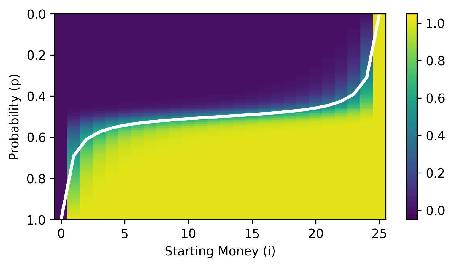
Figure 2: A visualization of the probabilities of player A winning the game given differing values of p, i, and N. The white line illustrates the mean probability for every value of i. Brighter colors illustrate a higher probability and darker colors illustrate a lower probability.
Looking at the above, it seems the more money in the game () the sharper the cutoff between the probabilities. This makes a lot of sense because winning by luck is less likely when there is more money in the game since more rounds are played. That is, given even the slightest edge in you’re almost guaranteed to win if is large and .
Monte Carlo Simulation
Just for fun, another thing we can do to validate our closed-form solution is to
compare it against a bunch of simulated games. You would assume that if we simulated
n_simulation games then as n_simulation approaches infinity that the ratio of
games that player A won would approach our analytical solution (Figure 3).
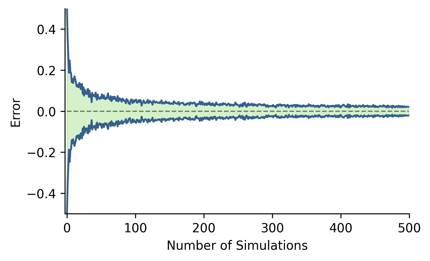
Figure 3: The error (RMSE) in the estimation of using the monte carlo simulation and the true probability using the analytical solution. Notice that as we increase the number of simulations ran, the average error decreases.
To do this, we need to first write code to simulate the playing of a game given the following variables:
- , the probability that player wins any independent round.
- , the amount of money player starts with.
- , the total amount of money in the game.
Below is the code to do that:
import random
from typing import Optional

class GamblersRuin:    def __init__(self, p: float, i: int, N: int) -> None:        self.p = p        self.i = i        self.N = N
        self.history = [i]
    @property    def ruined(self) -> bool:        if self.i <= 0:            return True
        return False
    @property    def won(self) -> bool:        if self.i >= self.N:            return True
        return False
    @property    def game_over(self) -> bool:        if self.ruined or self.won:            return True
        return False
    @property    def victor(self) -> Optional[int]:        if self.won:            return 1
        if self.ruined:            return 0
        return None
    def play_round(self) -> None:        if self.game_over:            print("Cannot play round, the game is over.")            return
        if random.uniform(0, 1) <= self.p: # Player A wins this round.            self.i += 1        else:            self.i -= 1
        # Keep track of the history of the game for analysis.        self.history.append(self.i)
    def play_game(self) -> int:        while not self.game_over:            self.play_round()
        return self.victor
Now that we have a way to simulate a single game, let’s simulate some number of
games and compute the probability of as the ratio of games that player A
won against the total number of games played. Therefore, the analog of the
true_probability() function for estimating the probability based on Monte
Carlo simulations would be:
def estimated_probability(p: float, i: int, N: int, n_sims: int = 1_000) -> float:    wins = []    for _ in range(n_sims):        game = GamblersRuin(p = p, i = i, N = N)        victor = game.play_game()        wins.append(victor)
    return sum(wins) / len(wins)
Now that we have both a closed-form and estimated solution to this problem, let’s compare the results of both using 1000 Monte Carlo simulations.
def compare(p: float, i: int, N: int, n_sims: int = 1_000) -> None:    true_p = true_probability(p, i, N)    est_p = estimated_probability(p, i, N, n_sims)
    print(f"p: {p:.02f} | i: {i} | N: {N:>3} | true: {true_p:.3f} | est: {est_p:.3f}")
compare(p = 0.50, i = 50, N = 100)compare(p = 0.49, i = 50, N = 100)compare(p = 0.49, i = 70, N = 100)compare(p = 0.40, i = 90, N = 100)
p: 0.50 | i: 50 | N: 100 | true: 0.500 | est: 0.510p: 0.49 | i: 50 | N: 100 | true: 0.119 | est: 0.115p: 0.49 | i: 70 | N: 100 | true: 0.288 | est: 0.262p: 0.40 | i: 90 | N: 100 | true: 0.017 | est: 0.018The results look really good! In general, both the estimated and true
probability seem to give very similar results (which is expected). Of course, as
we increase n_sims the difference between the true and estimated probabilities
should converge to each other.
Since we keep track of the histories of the game, one last thing we can do is plot the histories of each game. Doing so with 100 games, and the above settings gives:
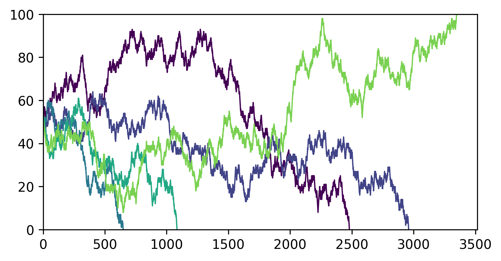
Figure 4: The history of 5 fair games played with parameters i = 50, N = 100, p = 0.5. Even though it was a fair game, player A still lost 4 games, tough luck. The colors represent each game played (5 total).
And this is pretty cool, you can see the random walk behavior clearly.
In summary, we explored the Gambler’s Ruin problem, a classic problem in probability theory where two players gamble until one player runs out of money. We derived a closed-form solution for the probability of one player winning the entire game, using both a clever brute force method and a more principled approach based on difference equations. This solution reveals how the initial stake, total money in play, and the probability of winning each round affect the overall chances of winning. Next, we implemented the game in Python, and ran a Monte Carlo simulation to experimentally validate the closed form solution. In doing so, we found that the closed-form solution and the Monte Carlo simulation provided similar results that converged upon increasing the number of simulated games. Finally, we ran an analysis to show how different values of initial parameters impacted the probability of one player winning, and also showed figures demonstrating the random-walk nature of these games.
References
- Blitzstein, J. (2013). Lecture 7: Gambler's Ruin and Random Variables | Statistics 110. Link
- Sigman, K. (2009). Gambler’s Ruin Problem. Link