Harmful Brain Activity Classification
The classification of harmful brain activity [1] [2] [3] [4] is one of the first steps in the effective diagnosis and treatment of neurological disorders [5] [6]. Today, electroencephalograms (EEGs) are used as non-invasive tests to record the electrical activity of the brain to detect various types of brain activity, harmful or otherwise. Although, manual labeling of EEG data is error-prone, subjective, and time consuming. For example, consider the scenario in which a patient undergoes a 24-hour EEG monitoring session resulting in a large amount of data being recorded across multiple electrode channels. Now, imagine a neurologist having to manually review all of this data, looking for subtle patterns that might indicate a seizure or other abnormal brain activity. It’s a tedious task, to say the least, and one that’s prone to fatigue, subjectivity, and error. Therefore, automation of this task is highly desirable to both reduce labeling error and speed up the labeling process. Doing so could improve the quality of life for both care teams and patients, and potentially even advance drug development.
A recent Kaggle competition, hosted by Harvard Medical School [7], challenged its competitors to do just this. That is, develop a model to classify various types of harmful brain activity, such as seizures, given EEG recordings from human patients. The dataset provided in this competition contained 6 types of harmful brain activity that were labeled by a varying number of expert annotators. In this article, we present our solution that we developed for this competition. We demonstrate that it was able to achieve 0.2625 ± 0.0233 KL-Divergence on high-quality samples, an AUC of 0.9274 ± 0.0272 on idealized samples, and ranked 60th out of 2767 other teams. Furthermore, we claim that our model makes minimal assumptions about the temporal length of the EEG, the number and spatial orientation of the EEG channels, and can be extended to include new modalities of data.
In the first section, we give a brief introduction to the background information needed to understand the task at hand. In the subsequent sections, we detail the competition data, and give an explanation of our solution. Finally, we give a discussion on the limitations of our model, talk about the competition itself, and mention some work on model interpretability. All of the code for this project is fully open source, reproducible, and can be found on GitHub.
Background
An electroencephalogram (EEG) is a non-invasive tool used to record electrical activity in the brain through electrodes that are placed on the scalp. These electrodes detect small voltage fluctuations resulting from ionic currents within the brain. Opposed to other neural recording devices, such as calcium imaging [8] [9], EEGs don’t have the resolution to capture the activity of single cells, but instead represent the summation of activity from large populations of neurons.
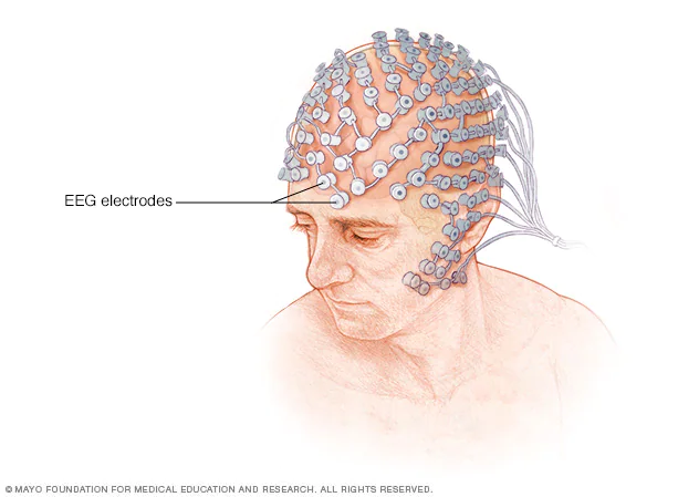
Figure 1: Graphical illustration of the EEG electrodes on the surface of the scalp.
The mechanism by which electrodes record ionic currents rely on volume conduction, the process by which electrical potentials are able to conduct (or travel) throughout tissue. When excitatory or inhibitory neurons fire (during an action potential), the extracellular voltage around the neurons change, and electrical fields are generated that propagate throughout the rest of the brain tissue. When these fields reach the surface of the scalp, and the adjacent electrodes, we are able to record the difference in potential created. Most of the signal recorded by EEGs is thought to come from pyramidal neurons in layers 3 and 5 of the cerebral cortex [10].
The placement of these electrodes on the scalp has been standardized, and there are a few commonly used layouts that we will cover. The most commonly used layout (or system) is the international 10-20 system (Figure 2). There are also the 10-10 and 10-5 systems, which are supersets of the 10-20 system that enable higher-density recordings.
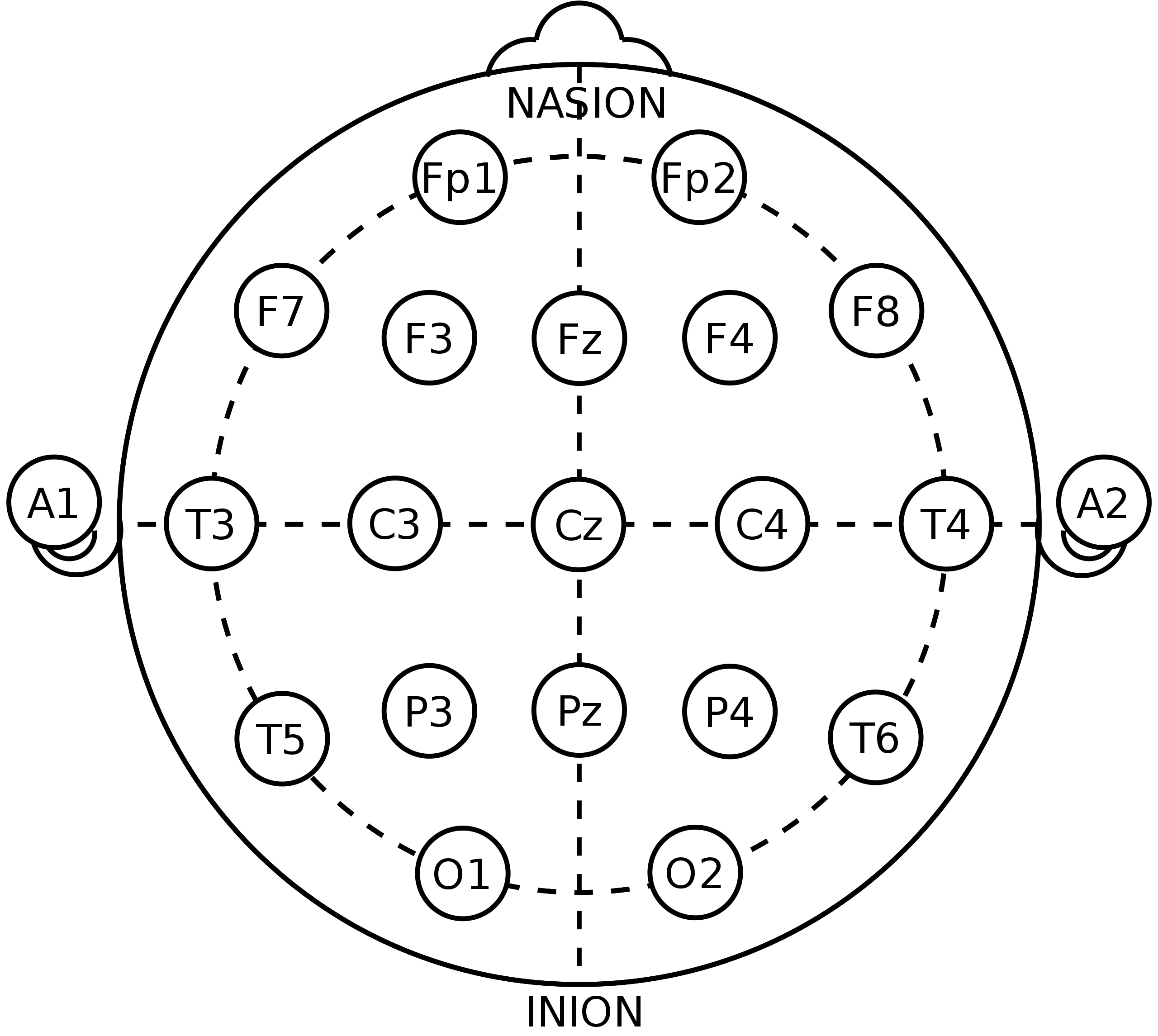
Figure 2: An illustration of the 10-20 system for EEG electrode placement. Notice that each electrode placement site has a letter to identify the lobe, or area of the brain, that it is located near: pre-frontal (Fp), frontal (F), temporal (T), parietal (P), occipital (O), and central (C).
When analyzing EEG signals, the raw signal from individual electrode channels are often processed to create what are called “montages”. A montage is a specific arrangement or combination of the electrode channels that helps highlight certain features of the underlying brain activity. One method of creating montages is through the computation of “bipolar channels.” These are created by subtracting the signal of one electrode from another. For example, a bipolar channel might be represented as Fp1-F7 (Figure 3), which means the signal from electrode F7 is subtracted from Fp1. This is helpful because it allows us to treat F7 as an estimate of the baseline activity for Fp1, and the process of subtracting F7 from Fp1 helps isolate the non-baseline activity from Fp1. Interested readers might consider reading a more detailed post about montages here.
It’s often that the primary signal we care about are the individual frequencies or oscillations of that signal. For this reason, you will often here about common frequency bands of interest, such as:
- Delta (0.5-4 Hz)
- Theta (4-8 Hz)
- Alpha (8-13 Hz)
- Beta (13-30 Hz)
- Gamma (>30 Hz)
There has been a lot of research around these frequency bands, linking them to various patterns of behavior. For example, delta activity is commonly seen in deep sleep states [11].
Data
For this competition, we were provided 106,800 labeled samples of data. At first glance, each sample consists of three modalities of data in the form of four spectrograms, the EEG signal from each electrode, and an EKG signal. These samples were given in the form of sections of 17,089 EEG/EKG recordings and 11,138 spectrograms. A single sample of data can be seen in Figure 3.
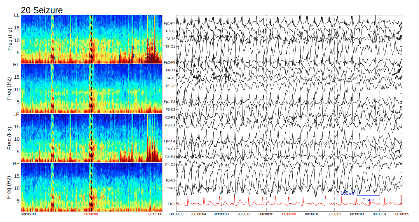
Figure 3: A single sample of data given for this competition. Notice that we were given 4 spectrograms (LL, RL, LP, RP) from the banana montage, EEG signals for each electrode (bipolar channels shown in above), and an EKG signal.
The specifics of each modality are listed below.
- 2D Spectrograms: We were provided four spectrograms for each sample, corresponding to the different chains of the double banana bipolar montage: left lateral (LL), right lateral (RL), left parasagittal (LP), and right parasagittal (RP). These spectrograms were computed from a 10-minute long EEG signal, contained frequencies up to 20 Hz.
- 1D EEG Signals: In addition to the 4 spectrograms, we were given 50 second long EEG signals recorded from electrodes placed in the 10-20 system. The recordings were sampled at 200 Hz, and were taken from the center of the larger 10-minute window that the spectrograms were computed from.
- EKG Signal: An electrocardiogram (EKG) signal was also provided, at the same frequency and length of the EEG signal.
Looking at the data, the results of the competition could answer interesting questions related to what modality of data is the most useful, and if combining modalities results in better performance. For example, we are given only 50 seconds of EEG recordings, but 10 minutes of spectrogram data (larger temporal window, but at a lower resolution). Is it that the more global information from the spectrograms, or high resolution information from the EEG signals, will give the best results?
The Labels
An important distinction to make is that although this competition is a classification competition, we are not given categorical labels for each sample. Instead, multiple expert annotators reviewed both the EEG and spectrogram data, then independently voted on the correct label. Therefore, the label that we are given are the votes of the multiple expert annotators, and we are instead tasked with predicting the distribution of expert annotator votes. To that end, we were scored with the KL Divergence metric, which is a distance metric used to compare two distributions. The KL-Divergence metric is computed as follows:
Where and are the predicted and ground truth labels respectively, which are normalized to have a sum equal to 1 in order to make them proper distributions.
What’s interesting about this metric, that may have unintended consequences, is that it is not commutative. That is, , where is the KL-Divergence between the distributions and . For these reasons, there were a couple comments on why other commutative metrics (such as Jensen-Shannon Divergence) weren’t used instead.
In the next 3 sections, we will explore important exploratory data analysis (EDA) findings that played a key role in guiding certain parts of our solution.
The Distribution of the Annotator Count per Sample is Bimodal
Plotting the distribution of the number of annotators that voted on each sample reveals a bimodal distribution (Figure 4). Looking closer at this distribution, it turns out that there are samples where the annotator count is between 1-7 and 10-28, but there are no samples where the annotator count is 8 or 9. This, I believe, hints at the true bimodality of the dataset.
Throughout the rest of this post, we will consider high quality samples to be those where the annotator count is greater than or equal to 10 (G10). Inversely, low quality samples are those where the annotator count is less than 10 (L10).
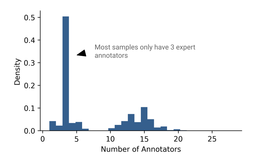
Figure 4: The distribution of the number of expert annotators per sample. Notice that the distribution is bimodal, and that most samples contain 3 expert annotators.
During the earlier weeks of the competition, people noticed that the public LB scores seemed to be significantly lower than local CV scores [13]. After some digging, it turns out that creating a validation set with only high-quality samples results in an almost 1:1 relationship between local CV and public LB. Given this information, there were a couple of extremely important things that we noted at the time:
- The public LB most likely contains high-quality samples, where the annotator count is greater than 9. Although we can’t know this for sure.
- If the public LB is composed of high-quality samples, it could be that the private LB has a larger subset of low-quality samples. If this is true, a big public-to-private LB shakeup could be expected if people overfit the public LB.
Some people [14] believed that we would see a large shakeup due to possibility number 2 listed above, and bet their whole solution on it. Because we were allowed to submit two solutions, we played it safe and had a submission optimized for each situation, as we’ll explain later.
There is a Varying Level of Annotator Agreement Per Sample
Given that we have multiple expert annotators reviewing the data, there are cases of disagreement in the correct label. Visualizing the level of agreement per sample reveals that most samples have 100% agreement, but that there are plenty of cases in which disagreement is present (Figure 5).
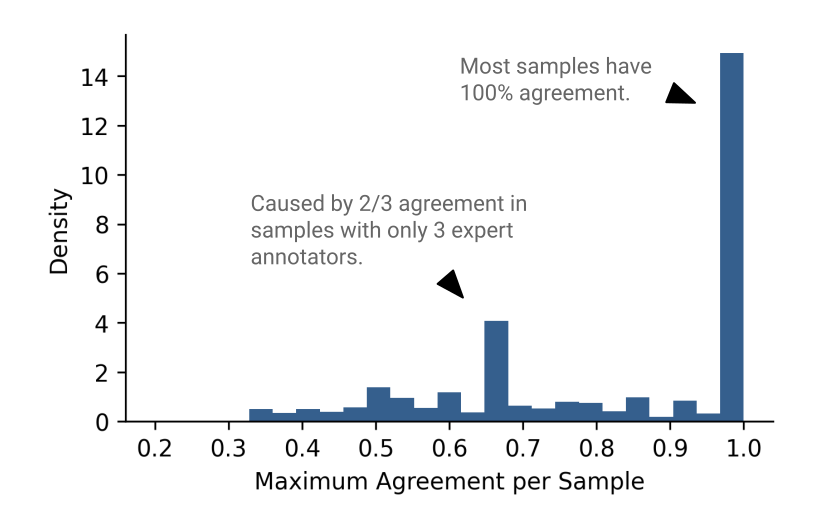
Figure 5: The distribution of annotator agreement per sample.
The hosts of the Kaggle competition gave a formal definition of the kinds of annotator agreement/disagreement, these names being: Idealized, Proto, and Edge. If your interested in reading more about how they define these, check out this link. Here, we will refer samples with at least 90% agreement as idealized samples, and samples with less than 90% agreement as non-idealized samples.
Methodology
For this competition, we benchmarked three models: Two unimodal models trained on the 1D EEG signals and the 2D spectrograms respectively, and a multimodal model that extends and combines the two previous models into a single model. We claim that the presented EEG model makes minimal assumptions about the temporal length of the EEG, the number and spatial orientation of the EEG channels, and can trivially be extended to include new sources and modalities of data.
Preprocessing
For preprocessing of the 1D EEG signals, we first computed the bipolar banana montage (excluding the EKG, Cz-Fz, and Pz-Cz channels). Then, each bipolar channel was temporally filtered with a Butterworth bandpass filter to remove frequencies outside the 0.25 to 50 Hz band. The resulting signal was then downsampled from 200 Hz to 50 Hz. Finally, we normalized the signal by the mean absolute deviation (MAD), and clipped the values to be between -10 and 10 to remove the presence of extreme values.
We chose to normalize by the MAD after finding the traditional standard deviation to not be a robust normalization factor due to the presence of large artifacts in some of EEG signals (Figure 6).

Figure 6: An example of a channel with large artifacts.
For preprocessing of the 2D spectrograms, we clipped the raw spectrograms between and , took the log, and then normalized each spectrogram to have mean 0 and standard deviation 1.
Model Architecture
At the beginning of this competition, we had a couple of properties that we wanted our model to satisfy. First, we would like it to not rely on the length of the EEG signal to make it robust to novel contexts. Next, we would prefer that it did not rely on the spatial orientation of the EEG electrodes, but could learn these relationships from the data during training. Finally, we wanted the model to work with minimally preprocessed data, and scale well.
To satisfy these properties, we took inspiration from some of the recent progress made in natural language processing, and decided to treat each spectrogram and EEG channel as a token that needs to be embedded into a single vector. After embedding each channel, we used an additive attention layer with learned positional encodings to route and mix the embeddings, effectively allowing us to learn the relationships between the different electrode channels without encoding it explicitly. In the last layer, we applied attention-pooling followed by a linear layer and softmax for classification.
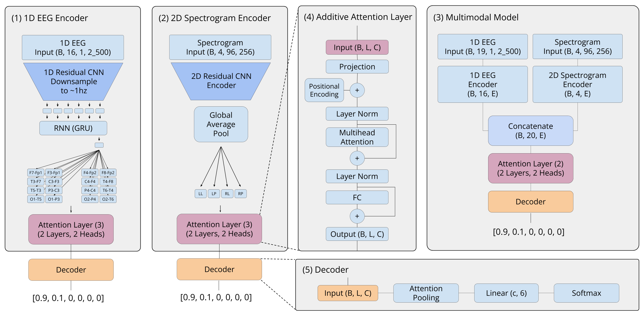
Figure 7: The architecture of the 1D EEG model (1), the 2D spectrogram model (2), and the multimodal model (3). As well as important blocks used, such as the additive attention layer (4) and the decoder (5).
Applying this framework in practice leaves one question: How do we embed each source of data into a vector in a manner that satisfies the properties previously mentioned?
To embed the 1D EEG channels, we used a CNN-RNN architecture that first stacks five 1D residual convolution blocks to simultaneously learn local features and downsample the preprocessed 50 Hz EEG channel to ~1 Hz. Afterwards, we use a recurrent neural network (RNN) within a many-to-one framework to temporally pool the signal into a single vector embedding. We claim that the use of an RNN for temporal pooling makes our model robust to the length of the EEG signal.
To embed the 2D spectrograms that are jointly provided with the EEG signals, we used a basic CNN architecture with ResNet-like encoder blocks followed by global average pooling. This architecture was again used to independently embed each of the 4 spectrograms provided (LL, LP, RL, RP).
The final multimodal model is an extension of both of the above architectures (see Figure 7). First, we take the embeddings of each EEG channel and spectrogram out of the previously discussed models (after the final attention layer, but before attention pooling), and then train an additional multi-layer additive attention layer on top of these embeddings to attend to every signal. We claim that this method could be modified to incorporate any modality of data, including text, assuming that you have a method of embedding the new data.
Cross-Validation (CV) Setup
Note:
CVis slang used in Kaggle to represent how you compute your score locally. Setting up a good local CV scheme is crucial to obtain a good score in a competition, since it reduces the number of times that you have to submit to the public LB. For example, if you had a local CV scheme that was perfectly linear with the public LB score, then you would rarely need to submit to the Kaggle public LB, and would essentially have infinite submissions. This allows for rapid testing of new ideas.
For our validation setup, we used a 10-fold GroupKFold on EEG ID, grouped by patient ID. We chose GroupKFold with these parameters because it ensures that out-of-fold (OOF) data only contains EEG recordings from patients who were not in the training set. This is advantageous because we believe the true test of generalizability is if a model can generalize to new patients. The testing set was chosen as the public LB in the Kaggle competition to ensure good alignment between local CV and public LB scores.
Training
For training, we developed a two-stage training scheme that takes advantage of the bimodal nature of the annotator count per sample (see Data). For the first stage, we trained on all of the data within the current fold for 20 epochs using the Adam optimizer with a static learning rate of 0.0003. In the second stage, we trained for 10 more epochs on just the high-quality samples, and reduced the learning rate to 0.0001. Beyond statically reducing the learning rate in the second stage, no learning rate schedulers were used. We used the KL-Divergence loss function, since it’s the metric we’re being tested on. Training was done in PyTorch on a NVIDIA GTX 1070 8 Gb GPU, and takes ~1 hour per fold. Therefore, the final submission took ~30 hours to train in total (3 models * 1 hour per model per fold * 10 folds).
For training augmentations on the 1D EEGs, we horizontally and vertically flip (p = 0.5) the ordering of the channels in the banana montage. Notice that when vertically flipping, you must also reverse the sign of the data because the order of subtraction in the bipolar channel changed. We also randomly zeroed out between 1-4 channels at a time with probability 0.5. For the 2D spectrograms, we only swapped the direction of the chains (both ll with rl and lp with rp).

Figure 8: The training loss of each model. The dotted line represents the transition from stage 1 to stage 2 of training. The high-quality and low-quality samples are plotted separately.
Minimal hyperparameter tuning was done. When evaluated on the testing set, single model performance demonstrated high variance, and so we chose an ensemble of 10 folds to combat against this high variance. Training for 20 and 10 epochs were conservatively chosen for stage 1 and 2 respectively, driven by earlier experimental observations that models had a tendency to converge around ~10 epochs in stage 1 and ~3 epochs in stage 2.
Results
We evaluate the results of the three models presented above with the KL-Divergence and AUC-ROC metrics, as shown in Table 1.
| Model | auc_all | auc_hq | auc_lq | kldiv_all | kldiv_hq | kldiv_lq |
|---|---|---|---|---|---|---|
| 1D EEG | 0.9203 ± 0.0317 | 0.9896 ± 0.0080 | 0.9364 ± 0.0368 | 0.6527 ± 0.0194 | 0.2757 ± 0.0214 | 0.8367 ± 0.0209 |
| 2D Spectrogram | 0.8731 ± 0.0422 | 0.9719 ± 0.0162 | 0.8866 ± 0.0612 | 0.8346 ± 0.0825 | 0.4284 ± 0.0278 | 1.0320 ± 0.1064 |
| Multimodal | 0.9274 ± 0.0272 | 0.9944 ± 0.0045 | 0.9408 ± 0.0330 | 0.6376 ± 0.0289 | 0.2625 ± 0.0233 | 0.8289 ± 0.0313 |
In summary, the 1D EEG model was the best performing unimodal model achieving an AUC Of 0.9203 ± 0.0317 on all of the idealized samples, and 0.9896 ± 0.0080 on the high-quality idealized samples. The 1D EEG model far outperformed the 2D spectrogram model on every metric, which achieved an AUC of 0.8731 ± 0.0422 on all of the idealized samples, and 0.9896 ± 0.0080 on the high-quality idealized samples. The multimodal outperformed both unimodal models, and was a small (but significant) improvement over the 1D EEG model by 0.0071 AUC on all of the idealized samples, and 0.0151 KL-Divergence on the high-quality samples.
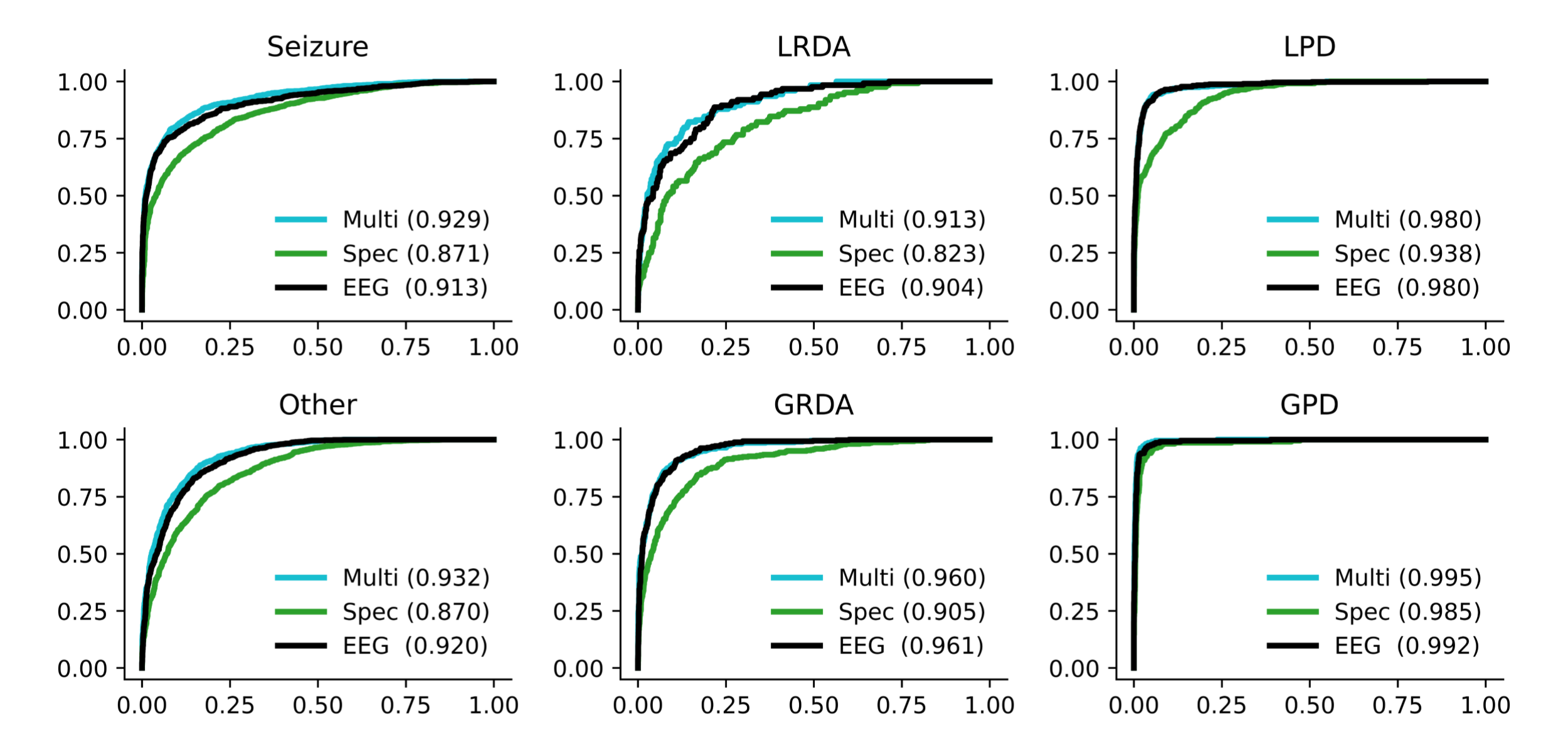
Figure 9: AUC curves shown for each model, and for each type of harmful brain activity. Results are only shown for idealized samples that had greater than or equal to 3 expert annotator votes.
Interpreting model performance, it seems that the higher temporal resolution of the 1D EEG model allowed it to outperform the 2D spectrogram model. Although, there also seems to be some amount of information contained within the 2D spectrograms that is not present in the 1D EEG signals, allowing the multimodal model to outperform both unimodal models.
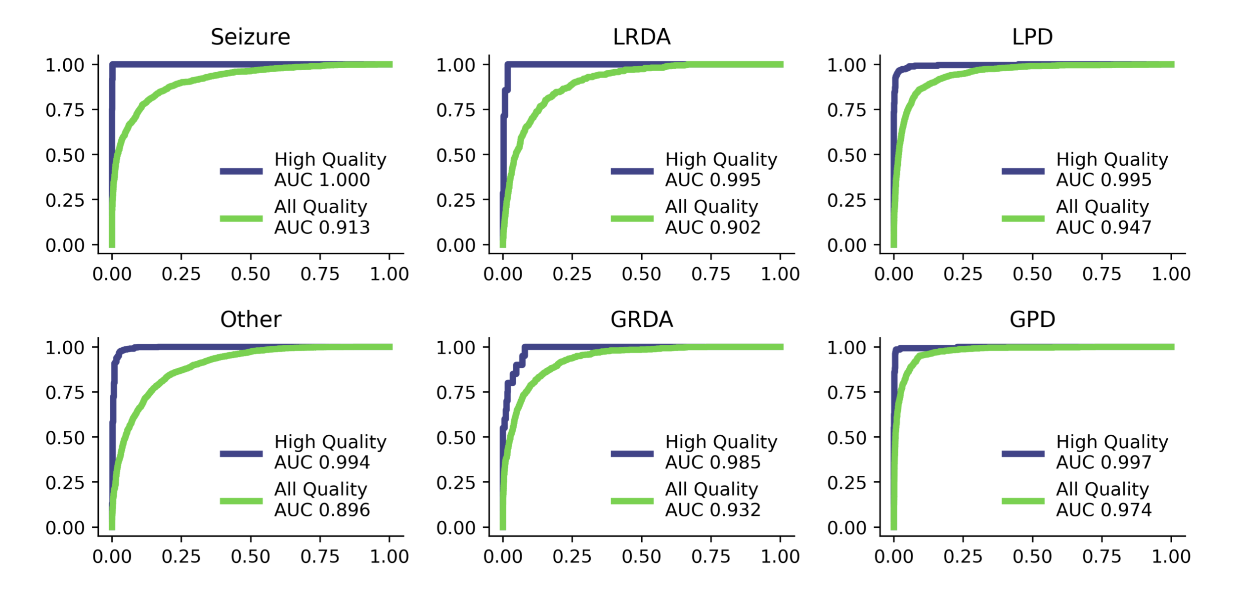
Figure 10: AUC curves from the multimodal model shown for each type of harmful brain activity, separated between low-quality and high-quality samples. Results only shown for idealized samples that had greater than or equal to 3 expert annotator votes.
Note the large gap in performance between the high-quality samples and the low-quality samples in the final evaluation and during training (Table 1 and Figure 9/10). We believe that this is for two reasons: First, there is more uncertainty in the labels of the low-quality samples as there are less expert annotators voting on the label. Second, the entropy of the ground truth labels are different in the low and high quality samples. That is, the low-quality samples are inherently low entropy because there is more sparsity in the labels, whereas the high-quality samples are higher entropy and less sparse leading to a distribution shift in the KL-Divergence metric. If the true cause of the difference in performance between high and low quality labels is a distribution shift in the entropy, one could likely fix this by adding a small constant epsilon to all of the low-quality samples to match the average entropy of the high quality samples. We did not test this.
For the kaggle competition, this solution ranked us 60th out of 2767 teams on the private LB with a KL-Divergence score of 0.338933. For reference, the first place winners (team Sony) won with a KL-Divergence score of 0.272332. Post-competition, we did not witness a large public-to-private LB shakeup, which we interpret to mean that both the public and private LB had a large sampling of high-confidence labels. Although again, we can’t know this for sure.
Discussion
In this post we presented an attention-style model to perform classification of harmful brain activity from EEG signals. We show that our multimodal model achieves 0.9274 ± 0.0272 AUC on idealized samples and 0.2625 ± 0.0233 KL-Divergence on high-quality samples. Furthermore, we claimed that our 1D EEG model is robust to the length of the EEG signal, the number of spatial orientation of the EEG electrodes, works with minimally preprocessed data, and scales well. With this model, we were able to rank 60th out of 2767 others teams in the Kaggle competition.
Although, our model is not without limitations. Specifically, we acknowledge the problem of interpretability. On this topic, we want to highlight the previous work by Barnett et al. [15] who proposed an interpretable solution that allows models to express their predictions in the form of “this looks like that”. We believe that this is a strong solution to the interpretability problem within the context of brain activity classification, and could benefit care teams.
In reading other competitors’ solutions [16] [17] [18] [19] [20] [21] [22], we realize that while our general architecture might be strong, the encoders themselves are fairly weak. We hypothesize that one could see significant improvements in performance by strengthening the encoders of both the 1D EEG and 2D spectrogram models.
We believe there are lots of room for improvement and new ideas, with some of the bigger ones being:
- Experiment with pre-training on other datasets (unsupervised and supervised).
- Changing the task from classification to a more real-time event-detection.
- Develop a library for rapid benchmarking of various machine learning models and ideas.
Code and data availability: The dataset used is publicly available and can be downloaded from the Kaggle website. The code for this project, and instructions for full reproducibility, can be found on GitHub. The final Kaggle notebook and models used can be found on Kaggle. All figures can also be reproduced (see Figures below).
References
- Huang, J.-S., Li, Y., Chen, B.-Q., Lin, C., Yao, B. (2020). An Intelligent EEG Classification Methodology Based on Sparse Representation Enhanced Deep Learning Networks. Link
- Nanthini, B. S., Santhi, B. (2017). Electroencephalogram Signal Classification for Automated Epileptic Seizure Detection Using Genetic Algorithm. Link
- Wagh, N., Varatharajah, Y. (2020). EEG-GCNN: Augmenting Electroencephalogram-Based Neurological Disease Diagnosis Using a Domain-Guided Graph Convolutional Neural Network. Link
- Thomas, J., Comoretto, L., Jin, J., Dauwels, J., Cash, S. S., Westover, M. B. (2018). EEG Classification Via Convolutional Neural Network-Based Interictal Epileptiform Event Detection. Link
- Behzad, R. and Behzad, A. (2021). The Role of EEG in the Diagnosis and Management of Patients with Sleep Disorders. Link
- Zheng X, Wang B, Liu H, Wu W, Sun J, Fang W, Jiang R, Hu Y, Jin C, Wei X and Chen SS-C (2023). Diagnosis of Alzheimer’s disease via resting-state EEG: integration of spectrum, complexity, and synchronization signal features. Link
- Jing, J., Lin, Z., Yang, C., Chow, A., Dane, S., Sun, J., Westover, M. B. (2024). HMS - Harmful Brain Activity Classification. Link
- Grienberger, C., Giovannucci, A., Zeiger, W. et al. (2022). Two-photon calcium imaging of neuronal activity. Link
- Jercog, P., Rogerson, T., & Schnitzer, M. J. (2016). Large-Scale Fluorescence Calcium-Imaging Methods for Studies of Long-Term Memory in Behaving Mammals. Link
- Britton JW, Frey LC, Hopp JLet al., authors; St. Louis EK, Frey LC (2016). Electroencephalography (EEG): An Introductory Text and Atlas of Normal and Abnormal Findings in Adults, Children, and Infants. Link
- Huang, H., Zhang, J., Zhu, L., Tang, J., Lin, G., Kong, W., Lei, X., & Zhu, L. (2021). EEG-Based Sleep Staging Analysis with Functional Connectivity. Link
- Evitan, G. (2024). Why shake-up didn't happen. Link
- Null, C. (2024). Whats with the CV in this comp?. Link
- Null, C. (2024). High Votes Distribution Wins!. Link
- Barnett, A. J., Guo, Z., Jing, J., Ge, W., Kaplan, P. W., Kong, W. Y., Karakis, I., Herlopian, A., Jayagopal, L. A., Taraschenko, O., Selioutski, O., Osman, G., Goldenholz, D., Rudin, C., & Westover, M. B. (2024). Improving Clinician Performance in Classifying EEG Patterns on the Ictal-Interictal Injury Continuum Using Interpretable Machine Learning. Link
- suguuuuu (2024). 1st place solution, team Sony. Link
- COOLZ (2024). 2nd place solution. Link
- Dieter (2024). 3rd place solution. Link
- YujiAriyasu (2024). 4th place solution. Link
- Vu Minh Quan (2024). 6th Place Solution for the HMS - Harmful Brain Activity Classification Competition. Link
- ishikei (2024). 9th Place Solution. Link
- T88 (2024). 11th Place Solution. Link
- Peters, R. (2024). 60th Place Solution: Single Multimodal Attention Model. Link
Figures
- EEG electrodes. Link.
- 10–20 system (EEG). Link.
- Single sample of data. Link.
- Custom. Number of annotators. Link.
- Custom. Distribution of agreement. Link.
- Custom. Example of artifact. Link.
- Custom. Model Architecture.
- Custom. Training loss. Link.
- Custom. Model performance (AUC). Link.
- Custom. Multimodal model performance on high/low quality samples (AUC). Link.
Tables
- Custom.