Principal Component Analysis
This post is a derivative of a talk that I gave at the ML@UMN club on April 25th, 2023. The original Kaggle notebook, and all of the associated code, for this talk can be found here. The goal of this talk (and this post) was to give a quick overview of vector projections, formally derive principal component analysis (PCA), and then go through a from-scratch implementation of PCA (in Python) within the context of performing dimensionality reduction of genotype data in hopes of being able to visualize some underlying latent structure of the high dimensional dataset.
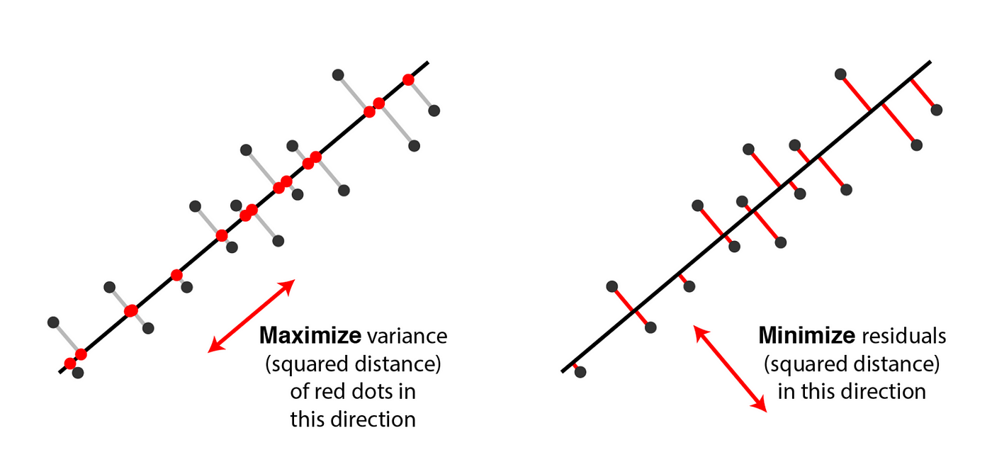
Principal component analysis (PCA) is an unsupervised method for dimensionality reduction. At a high level, this is done by finding vectors that point in the direction of maximum variance within our dataset, and then projecting our dataset onto these vectors. While PCA has many application, it’s commonly used to visualize high dimensional datasets in 2/3 dimensions, reduce noise (whitening), or as a preprocessing step for downstream applications.
Projections
As previously mentioned, PCA is performed by projecting our original dataset into a lower-dimensional subspace that preserves as much variance as possible. To do this, we must first talk about what is meant by a projection.
Assume that we have some dataset with samples and dimensions, that we want to project into a lower dimension. Also, let’s assume is mean centered (this doesn’t matter now, but will be important later on).
Now, let’s consider the case of projecting an arbitrary point in this dataset onto an arbitrary vector . Here the notation we will use will be to index the feature space, and to index the sample space.

Notice that we could do two kinds of projections. First, we could just get the scalar projection to find the distance along the projected point is (Figure 1 left), or we could find the vector in the direction of with magnitude equal to the scalar projection (Figure 1 right). Just by looking at the graph above, you should be able to convince yourself of the following equations:
Interpreting the above, given that the dot product of two vectors represent the amount of one vector in the direction of the other vector, this result intuitively makes sense. That is, the scalar projection is just the dot product of the vector given by the point and the unit vector .
The vector projection (inverse reconstruction of our data given projected data and vectors) is then:
Throughout the rest of this notebook we will make the assumption that the vector we are projecting our data onto is of unit length. This will be because we don’t care about the magnitude of , but only the direction, and making this assumption is important for later on. That is, . Under this assumption notice that the scalar projection just becomes the dot product, and the vector projection simplifies to (where for some ):
Minimization of Reconstruction Error
Now we are going to make the claim that minimizing the reconstruction error of our original data (where the reconstructed data is just the vector projection of our data onto some subset of vectors) is the same as maximizing the variance of the projected data.

To prove the statement above, notice that the reconstruction error is just the mean squared error (MSE) of the original dataset with our reconstructed dataset.
Which we want to minimize, thus:
Thus we have shown that minimizing the reconstruction loss is the same as maximizing the projection variance.
Principal Component Analysis (PCA)
So far we have defined what a projection is and shown that minimizing the reconstruction error of projected data is the same as maximizing the variance of the projected data. Intuitively, this is what PCA tries to capture. That is, we want to find the best vectors to project our data down onto, and have shown that these best vectors are the ones that maximize the variance of the projected data. Let’s try and solve for this formally:
But notice that to maximize this we could just make the vector we want to project onto arbitrary large, so we turn this into a constrained optimization problem. Another interpretation of this would be that we don’t care about the magnitude of , but only the direction, thus we constrain it’s magnitude to some fixed value (1 for simplicity).
Also notice that is just the covariance matrix assuming our data is mean centered (which was assumed when defining ). So we can make the substitution , then the problem becomes:
To solved these constrained optimization problems we use the Lagrangian multiplier to move the constraint into the optimization problem. This gives:
Now we need to solve for the stationary point (taking the gradient w.r.t. each variable and setting to zero). First, for the trivial case of we find:
And then for :
Now, because is the covariance matrix, and is symmetric, this is just the famous eigenvector problem. That is, are the eigenvectors of and are the eigenvalues. But what does this mean? This means that the vectors we want to project our data onto are the eigenvectors, with the largest eigenvalues, of the covariance matrix () of . This is because it turns out that the variance of our data onto some arbitrary eigenvector is just . Here is the proof if your interested:
Therefore as mentioned before, the eigenvectors with largest eigenvalues will be the vectors we will want to project our space onto because they will maximize the variance of our projected data. Furthermore, this is cool because it gives us a way to measure how much variance we have captured. If using all of the eigenvalues allows us to capture 100% of the variance, then the ratio of the sum of eigenvalues used to the total eigenvalues allows us to find out how much variance of the original dataset we have captured. This is an important quantification that will allow us to systematically capture 90% of the variance of our data (for example).
This gives us an algorithm for performing PCA on some dataset , and wraps up our derivation. To perform PCA and project your dataset onto dimensions, where , you do the following:
- Mean center the dataset.
- Compute the covariance matrix of the mean-centered dataset.
- Compute the eigenvalues and eigenvectors of the covariance matrix.
- Project your dataset (via a dot product) onto the eigenvectors with the largest corresponding eigenvalues.
Application: PCA on Genotypes
To bring this post full circle, let’s code a from scratch implementation of PCA (in Python) and use it to reduce the dimensionality of genotype data, to see if it’s possible to infer some underlying latent structure of the data.
Given that the genotype of any two individuals is roughly 99.6% alike [1], we would like to pick out what is different (the variants) and do dimensionality reduction on those parts of the genome. Today, we identify these genetic variants through a process called variant calling. In this post, the dataset we will be using is from the 1000 Genomes Project [1] and is given in the form of a VCF (Variant Call Format) file, containing variants at various loci on an individual’s chromosome. Such variants include single nucleotide polymorphisms (SNPs) or structural variants (SVs) such as insertion/deletions (INDELs) and more.
This application was inspired by Maria Nattestad’s YouTube video [3] and implementation of this same project. Although, we believe this idea was originally based off of this paper [2], all of which can be found in the references links.
For the dataset used in this post, we will be using a different dataset than the original paper and a different chromosome of the same dataset that Maria Nattestad used in her implementation. If you are following along, we also recommend you use a different dataset, or the same dataset and a different chromosome, than either Maria Nattestad (Chr 22) or this post (Chr 21) uses.
Also, this post does not include any of the functions to load/process the dataset. If your following along, make sure to follow along from the notebook on my GitHub.
Now, let’s extract the important information from the VCF files, including the allele’s and information about the population we sampled from.
vcf_dir = "path to VCF dir"panel_dir = "path to PANEL dir"
samples, genotypes, variant_ids = allele_indices(vcf_dir, skip_every)population_map, superpopulation_map = parse_panel(panel_dir)
# Find the superpopulation of each sample.superpopulation = pd.Series(samples).map(superpopulation_map)
genotypes = np.array(genotypes) # shape: (samples, variant_count // skip_every, 2)genotypes = np.sum(genotypes, axis = 2)
# Reduce size due to compute constraints.genotypes_small = genotypes[::10]
# Number of alleles (m): 2076# Number of samples (n): 1092m, n = genotypes_small.shape
We will strictly follow the above mentioned procedure to perform PCA. First, we must mean center the dataset.
# Calculate and subtract the mean.mean = np.mean(genotypes_small, axis = 1, keepdims = True)
genotypes_normalized = genotypes_small - mean
Next, we compute the covariance matrix of the dataset (ether dividing by n-1 or n, we will use n-1).
covariance = genotypes_normalized.dot(genotypes_normalized.T) / (n - 1)Next, compute the eigenvectors and eigenvalues of the covariance matrix. Luckily for us, NumPy sorts them automatically. This will make the selection step easier.
eig_values, eig_vectors = np.linalg.eigh(covariance)
# They are in ascending order, we want the opposite.eig_values = eig_values[::-1]      # shape (2076,)eig_vectors = eig_vectors[:, ::-1] # shape (2076, 2076)
As a side note, let’s test how much variance is captured by selecting more and more components.
np.cumsum(eig_values / np.sum(eig_values))[0:10]array([0.0831045 , 0.13070515, 0.14289654, 0.15236331, 0.16062823, 0.16877235, 0.17622259, 0.18349874, 0.19060836, 0.19756033])We can see that by taking n_components=1 then we will capture 8.3% of the
variance of the original dataset, by taking n_components=2 then we will
capture 13.1% of the variance, and so on.
For visualization purposes, let’s take n_components=2. The eigenvalues are
already sorted in descending order. Because the covariance matrix is positive
semi-definite, s = d.T, and we can just take the leading two principal
components straight from s.
pc1 = eig_vectors[:, 0]pc2 = eig_vectors[:, 1]Now we do a change of basis of our original dataset with our PC1 and PC2 forming the new subspace. This is the final “dimensionality reduction” step. Because the eigenvectors are of normal length, projecting out data onto this space is just a simple dot product.
pc1_plot = genotypes_normalized.T.dot(pc1)pc2_plot = genotypes_normalized.T.dot(pc2)Now lets visualize the reduced dataset.

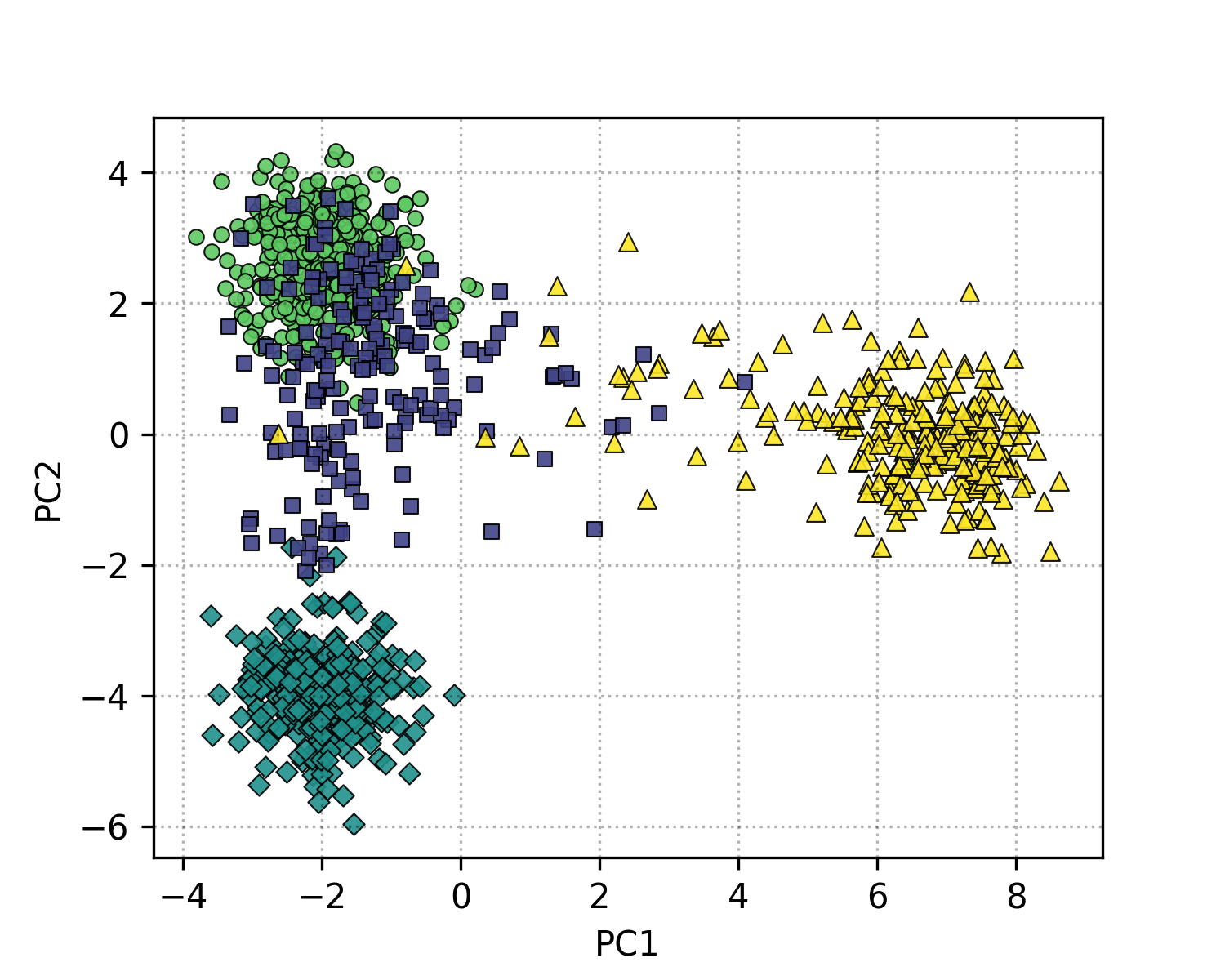
Figure 3: Genotype data projected onto PC1 and PC2, colored by the superpopulation code.
In Figure 3, each point represents an individual (sample), colored by their superpopulation. From this, we can see a clear clustering of individuals based on their genetic ancestry, with distinct groupings corresponding to different superpopulations (Europe, Asia, America, and Africa). This demonstrates how PCA can be used to visualize underlying high-dimensional latent structure in 2 dimensions, which only captures about 13% of the total variance.
We can also compare this with the scikit-learn PCA implementation to verify to ourselves that what we have done is correct. Additionally, in the notebook we performed an unsupervised clustering step. If your interested in checking these out, check out my GitHub.
In this post, we introduced principal components analysis (PCA) as a method for unsupervised dimensionality reduction, formally derived PCA from first principals, and applied it to a real-world genomic dataset to infer underlying high-dimensional latent structure.
Full examples can be found on my GitHub.
References
- The 1000 Genomes Project Consortium (2015). A global reference for human genetic variation.. Link
- Novembre, J., Johnson, T., Bryc, K., Kutalik, Z., Boyko, A. R., Auton, A., Indap, A., King, K. S., Bergmann, S., Nelson, M. R., Stephens, M., & Bustamante, C. D. (2008). Genes mirror geography within Europe. Link
- Nattestad, M. (2021). Genes and geography -- a bioinformatics project. Link