The Rosenblatt Perceptron Algorithm

The Perceptron algorithm is one that’s close to my heart. It was the first machine learning algorithm that I learned, while taking MITx’s 6.036 with Leslie Kaelbling, and it’s possibly the reason I am in this field today. In this post, I explore the Perceptron algorithm, its history, and implement it in Python. Given that this algorithm is commonly taught as an introductory topic, I will also provide a little bit of background on hyperplanes and binary classifiers to hopefully inspire readers who might be just starting their machine learning journey. That said, I do assume a sufficient understanding of introductory linear algebra topics.

Data Separation

Before we dig into the Perceptron algorithm itself, it’s important to understand the task we are trying to solve. More specifically, I will attempt to answer what exactly a “binary classifier” is, and the formal mechanism by which “data separation” is performed (via a hyperplane). These ideas are crucial to understand what the Perceptron algorithm is trying to solve, and how it does what it does.

A binary classifier is a function, mapping individual samples of data to a binary label. Mathematically, it’s a function $f$ of the form:

f: x \to \{0, 1\}

Where $x$ is a sample of data. The classical example of this is a spam classifier, where each sample of data is an email and the output is the binary label 0 if the email is not spam, or 1 if the email is spam.

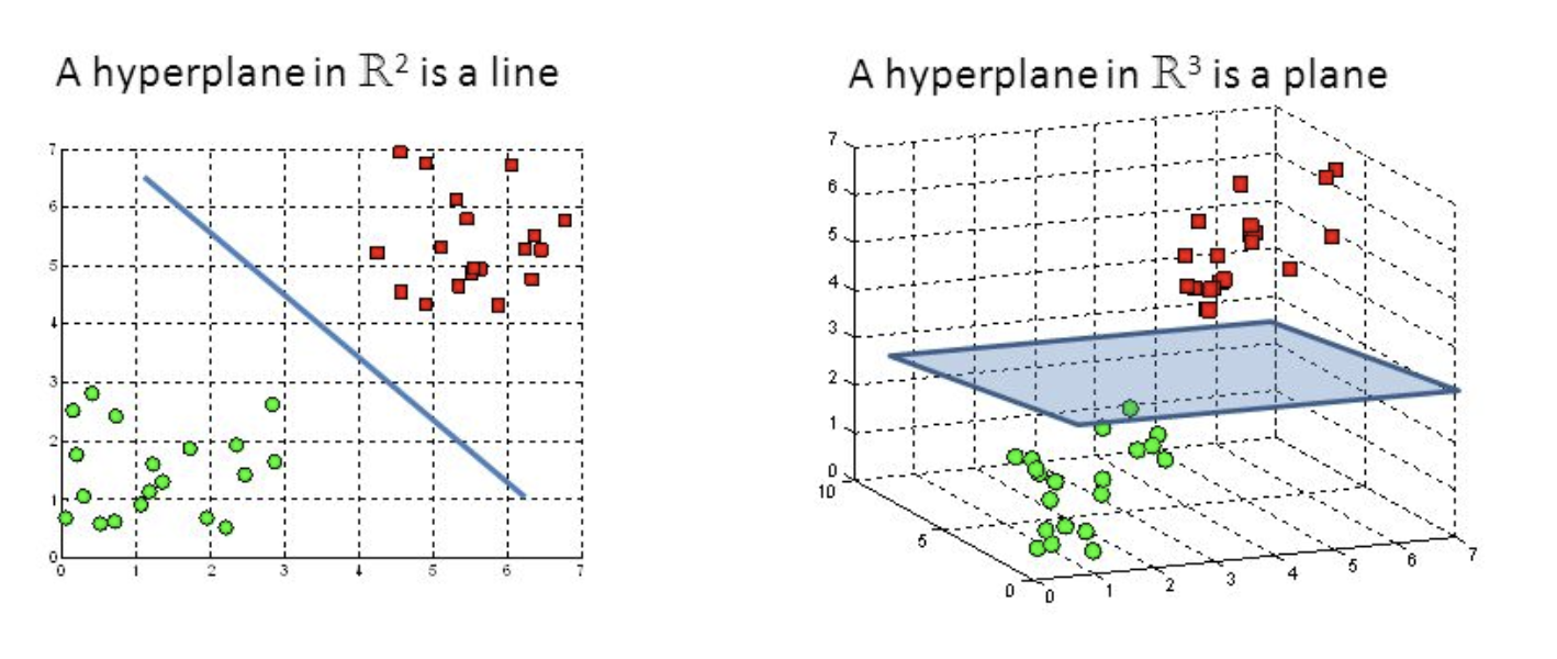
**Figure 1:** Demonstration of a hyperplane. In two dimensions, a hyperplane is a line. In three dimensions, a hyperplane is a plane.

Now that we understand what a binary classifier is, what is the formal mechanism by which we separate data into two classes? To understand this mechanism of data separation, one must first understand the idea of a hyperplane. Within the context of data separation, a hyperplane is a boundary that separates a euclidean space into 2 parts (Figure 1). To add intuition to this:

In 2D, a hyperplane is a line that splits the plane into two parts.
In 3D, a hyperplane is a plane that splits the space into two parts.
In nD (n > 3), a hyperplane is an (n-1)-dimensional subspace that splits the n-dimensional space into two parts.

Mathematically, a hyperplane can be described by the equation:

\theta_0 + \theta_1 x_1 + ... + \theta_d x_d = 0

\begin{equation} \theta_0 + \theta^{\top} x = 0 \end{equation}

Here, $x = (x_1, ..., x_d)$ represents a point in d-dimensional space, $\theta = \left\langle \theta_1, ..., \theta_d \right\rangle$ is the normal vector to the hyperplane, and $\theta_0$ is the bias term. The points $x$ that satisfy equation (1) are the points that lie on the hyperplane. One of the key features of a hyperplane is its ability to separate points in space since points that lie on the positive side of the hyperplane satisfy $\theta_0 + \theta^{\top} x > 0$ , while points on the negative side satisfy $\theta_0 + \theta^{\top} x < 0$ . This property allows us to define a binary classifier as:

\mathrm{sign}(\theta_0 + \theta^{\top} x)

This is the formal mechanism by which data separation occurs.

The Perceptron Algorithm

The Perceptron algorithm, formulated by Frank Rosenblatt with inspiration from earlier work done by Warren McCulloch and Walter Pitts, is an algorithm for supervised learning of a binary classifier (pre-gradient descent). More specifically, given some set of weights $\theta$ and a bias $\theta_0$ , it describes a method for training a linear classifier $h(x ; \theta, \theta_{0})$ of the form:

\begin{equation} h(x ; \theta, \theta_0) = \mathrm{sign} (\theta^{\top} x + \theta_0) = \left\{ \begin{array}{ll} +1 & \text { if } \theta^{\top} x+\theta_{0}>0 \\ -1 & \text { otherwise } \end{array} \right. \end{equation}

Given this formulation of the binary classifier that we aim to learn, the Rosenblatt Perceptron algorithm describes the following procedure for finding possible values of $\theta$ and $\theta_0$ to separate some dataset:

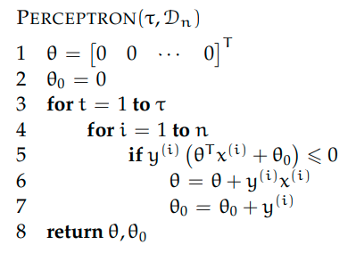
**Figure 2:** The (Rosenblatt) Perceptron algorithm.

What’s quite amazing about the Perceptron algorithm is that if a dataset is linear separable, then the Perceptron algorithm can be proven to always converge and be able to find a $\theta$ and $\theta_0$ that separates the dataset. Furthermore, the proof also reveals an upper bound on the number of steps that the Rosenblatt Perceptron Algorithm will take to converge. We’ll present the proof of this in a later section.

History and The AI Winter

The story of The Perceptron begins with Warren McCulloch and Walter Pitts back in 1943 when they published an article titled “A logical calculus of the ideas immanent in nervous activity” [2]. This article formulated the idea for a biologically-inspired “fictitious net” based on a set of assumptions about the properties of individual neurons, populations of neurons, and the anatomical structure of the brain. This early model, while groundbreaking at the time, had its limitations. For example, their formulation was done using propositional logic and assumed neuronal inputs/outputs (IO) were binary, which we know today not to be true. Regardless, this work would lay the initial foundation for the next couple decades of work in artificial intelligence.

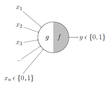
**Figure 3:** A diagram of the McCulloch and Pitts Perceptron. Notice that the input and output are both binary.

The next piece of development came in 1949 after Donald Hebb published a book titled “The Organization of Behavior” [3]. In this book, Hebb introduced a theory of synaptic plasticity [4] [5] often described as “neurons that fire together, wire together.” This theory states that neurons could strengthen the connections between each other through repeated activation. More formally, Hebb proposed that if a neuron consistently takes place in causally firing another neuron, the synaptic efficiency between the two neurons would increase. Today, this concept is known as Hebbian Learning or Hebb’s Rule. As a corollary, this means that the strength of connection between two neurons can change over time as a function of learning and/or experience. This highlights the idea of neuronal activity as a weighted function of it’s inputs–rather than a binary one–and learning as a change in these synaptic weights. That is, it provides a mechanism by which neurons could learn as a function of data (via modifying their synaptic weights to fit the data), a concept that will prove important in the further development of artificial neural networks.

Frank Rosenblatt, while working at Cornell with funding from the US Office of Naval Research, built on the foundations of Hebb and extended McCulloch and Pitts’ work to model the Perceptron’s output as a weighted sum of it’s inputs. Furthermore, he built a hardware implementation to test out his new idea in practice. His work was officially released in 1957 when the Mark 1 Perceptron (Figure 4) was announced, and the release of his subsequent paper “The perceptron: A probabilistic model for information storage and organization in the brain” [6] one year later.

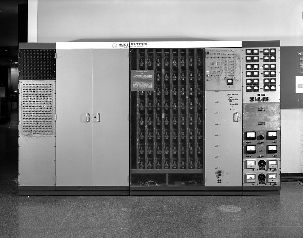
**Figure 4:** An image of the Mark I Perceptron. It is currently located at the Smithsonian, where it was transferred to from Cornell in 1967.

With Rosenblatt’s work published, there was a lot of attention around this new idea, both positive and negative. Even with the skeptics, Rosenblatt was very confident in his work, and made the claim that Perceptrons should be able to learn arbitrary functions (basically foreshadowing the next 60 years of AI development). Unfortunately, his work still had some missing parts that would soon be highlighted.

One of the skeptical parties, Minsky and Papert, released a famous book in 1969 titled “Perceptrons: an introduction to computational geometry” [7]. In this book, they provided a rigorous mathematical analysis of the Perceptron’s capabilities and limitations. Notably, they proved that it was impossible for (a one layer) Perceptron model to learn the XOR function, a simple logical operation that requires nonlinear separation (Figure 5).

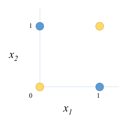
**Figure 5:** An illustration of the XOR function. A XOR function is a simple logical operation that requires non-linear separation.

What’s often left out of this story is that Minsky and Papert’s book wasn’t entirely negative. In it, they also discussed the concept of multi-layer Perceptrons, which could theoretically learn the XOR function, and solve the previous limitations of single-layer models. However, at the time there was no effective method for training such multi-layer models.

After this publication, the money dried up, and interest died out. The first so-called AI winter had begun. Even worse, Rosenblatt unexpectedly died on July 11, 1971 (his 41st birthday) in a boating accident on the Chesapeake Bay, and wasn’t able to witness the revival of his ideas some years later.

Convergence Theorem

Getting back to the Perceptron algorithm itself, what’s quite amazing is that if a dataset is linear separable, then the Perceptron algorithm can be proven to always converge and be able to find a $\theta$ and $\theta_0$ that separates the dataset. In order to do so, we first have to make a couple of assumptions (stated below), then follow a rather clever line of reasoning. Most, if not all, of my work will be deviations from the original Fall 2019 6.036 class notes [1] and various other online sources [8] [9].

Theorem: First, let’s make the following assumptions:

Linear separability: There exists a parameter $\theta^*$ and a $\gamma > 0$ such that for all values of $i = 0, 1, \ldots, n$ that $\frac{y_i (\theta^{*T} x_i)}{|| \theta^* ||} \geq \gamma$ . (hint: $\theta^*$ is our final solution that we want to find)
That all of the data points have a bounded magnitude of $|| x_i || < R$ for all $i = 0, 1, \ldots, n$ .

Then the Perceptron algorithm will not converge for at most $(\frac{R}{\gamma})^2$ steps (most other resources phrase this as the algorithm will make at most $(\frac{R}{\gamma})^2$ mistakes or errors).

Note: Let’s think about why this theorem proves that the Perceptron algorithm guarantees convergence. Well… if we know that the model will not convert for at most $(\frac{R}{\gamma})^2$ steps, then we have an upper bound on when the model will converge. Thus, if $(\frac{R}{\gamma})^2$ is finite and the original two assumptions hold, then we can guarantee that the model will converge in less than $(\frac{R}{\gamma})^2$ steps.

Proof: To start this proof, let $\theta^{(k)}$ be the parameters of the model at iteration $k$ of the algorithm. Notice that with this notation we let $\theta^{(0)} = 0$ . That is, the parameters of the model at iteration 0 are set to 0 manually by us from equation (1).

A high-level overview of the proof goes as follows: We want to derive both a lower and upper bound on $\frac{\theta^*}{|| \theta^* ||}$ .

In this proof, our goal is to find some upper bound on $k$ . Because if we can do so then we can prove that the model will make at most $k$ iterations before convergence.

To start the proof, let’s look at the $\frac{\theta^{(k)} \theta^*}{|| \theta^* ||}$ .

\begin{aligned} \frac{\theta^{(k)} \theta^*}{|| \theta^* ||} &= \frac{(\theta^{(k-1)} + y_i x_i) \theta^*}{|| \theta^* ||} \\ &= \frac{\theta^* \theta^{(k-1)} + \theta^* y_i x_i}{|| \theta^* ||} \\ &= \frac{\theta^* \theta^{(k-1)}}{|| \theta^* ||} + \frac{\theta^* y_i x_i}{|| \theta^* ||} \\ &\geq \frac{\theta^* \theta^{(k-1)}}{|| \theta^* ||} + \gamma \\ \end{aligned}

Now, notice the recursive pattern here on the left side of the equation we just derived. Applying the same logic we derived above to the left side of the equation we can see the pattern above reduce into the following:

\begin{aligned} \frac{\theta^{(k)} \theta^*}{|| \theta^* ||} &\geq \frac{\theta^* \theta^{(k-1)}}{|| \theta^* ||} + \gamma \\ &\geq (\frac{\theta^* \theta^{(k-2)}}{|| \theta^* ||} + \gamma) + \gamma \\ &\geq ((\frac{\theta^* \theta^{(k-3)}}{|| \theta^* ||} + \gamma) + \gamma) + \gamma \\ &\geq k \gamma \\ \end{aligned}

Now that we have this, let’s do some analysis on the left side of the equation as currently it is not quite clear how it relates to our original goal.

One trick we’ll use is that, by the Cauchy–Schwarz inequality, the inner product of two vectors is less than or equal to the individual magnitudes of the vectors multiplied together. Using this fact, we can make the following simplification of the left side.

\begin{aligned} \frac{\theta^{(k)} \theta^*}{|| \theta^* ||} &\leq \frac{|| \theta^{(k)} || \; || \theta^* ||}{|| \theta^* ||} \\ &\leq || \theta^{(k)} || \\ \end{aligned}

Thus by this logic:

\begin{aligned} || \theta^{(k)} || &\leq k \gamma \\ \end{aligned}

And this is part one of the proof. In the high level overview I mentioned that we wanted to derive both an upper and lower bound for $\theta^*$ , and now we just have the lower lower bound left to do.

Now to derive the lower bound:

\begin{aligned} || \theta^{(k)} ||^2 &= || \theta^{(k-1)} + y_i x_i ||^2 \\ &= || \theta^{(k-1)} ||^2 + 2 y_i \theta^{(k-1)^T} x_i + || x_i ||^2 \\ &\leq || \theta^{(k-1)} ||^2 + || x_i ||^2 \\ &\leq || \theta^{(k-1)} ||^2 + R^2 \\ \end{aligned}

Note that the step on line 2-3 above is possible because $2 y_i \theta^{(k-1)^T} x_i \leq 0$ . That is because the algorithm is known to have made a mistake on the datapoint $x_i$ (by the if-statement in the algorithm).

Then by a very similar recursive reasoning done above we get the following:

\begin{aligned} || \theta^{(k)} ||^2 &\leq k R^2 \\ \end{aligned}

And now we are basically done, just compare this equation with the previously derived equation to see that the following is indeed the case.

\begin{align*} k^2 \gamma^2 &\leq || \theta^{(k)} ||^2 \leq k R^2 \\[5pt] k^2 \gamma^2 &\leq k R^2 \\[5pt] k &\leq \frac{R^2}{\gamma^2} \\ && \blacksquare \\ \end{align*}

And that’s it for the proof.

Implementation

To bring the discussion of the Perceptron algorithm full circle, let’s implement it in Python using NumPy. Here, I’ll show the core of the algorithm, but all of the code used to generate the following figures and data can be found here.

def perceptron(x: np.ndarray, y: np.ndarray, max_steps: int = 10_000):
    sample_size, num_dims = x.shape

    # Initialize theta and theta_0 to zeros.
    th = np.zeros((num_dims,))
    th_0 = np.zeros((1,))

    for t in range(max_steps):
        has_error = False # Flag for convergence.

        for i in range(sample_size):
            if y[i] * (np.dot(x[i], th) + th_0) <= 0:
                th = th + (y[i] * x[i])
                th_0 = th_0 + y[i]

                has_error = True

        if not has_error: # Early stopping for convergence
            break

    return th, th_0

It’s a pretty simple algorithm at its core, and should generalize to arbitrary dimensions (n>2). Additionally, I added a couple of lines for early stopping if the model converges before the maximum number of steps allowed is reached. With the algorithm implemented, let’s test it against a couple of toy datasets created from the scikit-learn library.

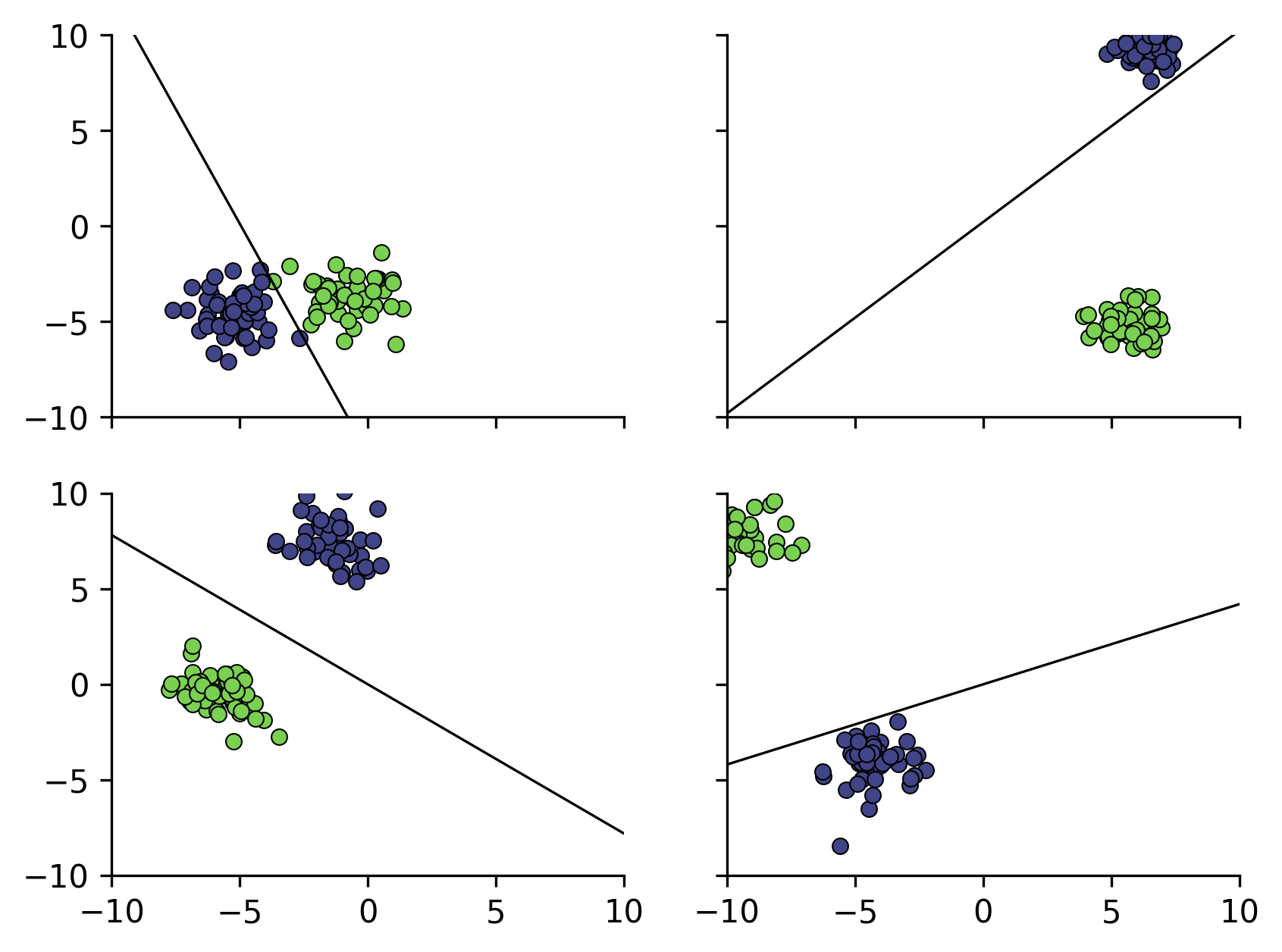
**Figure 6:** An example of the Perceptron algorithm on different toy datasets. The left 2 images illustrate good fits that would likely generalize quite well, and the right 2 illustrate proper data separation but a poor fit.

As we can see the Perceptron Algorithm found a $\theta$ and $\theta_{0}$ that separates the data, even in the hardest case that I could find (top left image).

Beyond the Perceptron

While the Perceptron algorithm works well in the cases presented above (left side), there are a couple of limitations. For one, the Perceptron algorithm is quite sensitive to outliers. For example, because the Perceptron algorithm only guarantees convergence if the dataset is linearly separable, even a single outlier can cause the Perceptron algorithm to never converge. Additionally, because the Perceptron algorithm stops as soon as it’s finds a hyperplane, there is no guarantee on how good the hyperplane it will find is (depending on how you choose to define a good hyperplane). For example, look at the hyperplanes found by the Perceptron algorithm in the right side of Figure 6. These models would likely have a hard time generalizing to new data because of how close the hyperplane is to the blue samples.

The limitations of the Perceptron algorithm, particularly its inability to find an “optimal” hyperplane, leads us to more advanced algorithms. One such algorithm is the Support Vector Machine (SVM), which not only finds a separating hyperplane, but tries to find a hyperplane that maximizes the margin between the two classes. Furthermore, SVMs can be made to be less sensitive to outliers, and can also be combined with kernels to handle non-linear data separation. If you’re interested in learning more about SVMs and how they improve upon the Perceptron, check out my detailed explanation of hard-margin SVMs here.

In conclusion, we introduced the idea of a binary classifier and described the formal mechanism by which data separation occurs. Next, we described the Perceptron algorithm, gave a recap of its history, and proved that it will always converge if the dataset is linearly separable. Finally, we implemented the algorithm in Python, tested it on toy data, talked about it’s limitations, and mentioned SVMs as a more modern solution.

References

Kaelbling, L. (2020). 6.036 Lecture Notes. Link
McCulloch, W.S., Pitts, W. (1943). A logical calculus of the ideas immanent in nervous activity. Link
Hebb, D. O. (1949). The organization of behavior; a neuropsychological theory.. Link
Citri, A., Malenka, R. (2008). Synaptic Plasticity: Multiple Forms, Functions, and Mechanisms.. Link
Magee JC, Grienberger C. (2020). Synaptic Plasticity Forms and Functions. Link
Rosenblatt, F. (1958). The perceptron: A probabilistic model for information storage and organization in the brain. Link
Minsky, M., Papert, S. A. (1988). Perceptrons: An Introduction to Computational Geometry. Link
Collins, M. (2012). Convergence Proof for the Perceptron Algorithm. Link
(2023). Exploration 2.4: Perceptron Convergence Theorem and Proof. Link

Figures

Image of a hyperplane in 2/3 dimensions. Link.
Image of the Rosenblatt Perceptron Algorithm from MITx 6.036 notes. Link.
McCulloch and Pitts’ Perceptron. Link.
The Mark I Perceptron. Link.
The XOR function. Link.
Four examples of the Perceptron fit. Link.