Phase Transitions & The Ising Model
I recently made a small foray into statistical mechanics while trying to understand the critical brain hypothesis [1] [2] [3]. Including what exactly it means for the brain to operate near a 2nd-order phase transition, and why the observation that the size and lifetime distributions of neuronal avalanches are power-law distributed offers experimental support for criticality. This lead me down a pretty deep rabbit hole of ideas in statistical mechanics such as the scaling hypothesis, mean-field theory, and the renormalization group. Some of which I will explore in this post.
This post on phase transitions and the Ising model is going to be one in a couple of posts I hope to make on topics at the intersection of physics, neuroscience, and machine learning. These topics include (but are not necessarily limited to) free energy and entropy, Hopfield networks, Boltzmann machines, and the critical brain hypothesis. The discussion of the Ising model in this post will give a smooth transition into a future post on Hopfield networks, which are energy-based models of associative memory built on top of the Ising model. That said, these posts are momentarily in competition with a bunch of mechanistic interpretability posts I also want to get up soon.
To give a high level overview of this post, we will first cover some background information on what a phase transition is and its classifications. Introduce critical exponents, the scaling hypothesis, and the concept of universality observed between different models. Then, we will discuss the Ising model, a model of magnetism at the scale of the magnetic dipole moment of an electron, in a varying number of dimensions. We will discuss what it means to solve a thermodynamic problem, namely computing the free energy and it’s various derivatives, then solve the Ising model in zero- and one-dimensions. Finally, we will cover the mean field approximation of the Ising model in -dimensions, talk about when this approximation does and does not hold, and provide a very interesting link between mean-field theory and variational inference in Bayesian statistics.
Phase Transitions
A phase transition is an event, that occurs when small changes in a control parameter (such as temperature) lead to large, and sometimes discontinuous, change in the macroscopic properties of a system in the thermodynamic limit. These macroscopic properties are often referred to as order parameters (such as magnetism, see Figure 2). Using the Ehrenfest classification, phase transitions are further classified by the system’s free energy, where -th-order phase transitions involve a discontinuity in the -th partial derivative of the free energy with respect to the order parameter. But, throughout this post we will only distinguish between discontinuous (first-order) and continuous (2nd-order and above) phase transitions. This distinction can be seen more clearly in Figure 1 below.
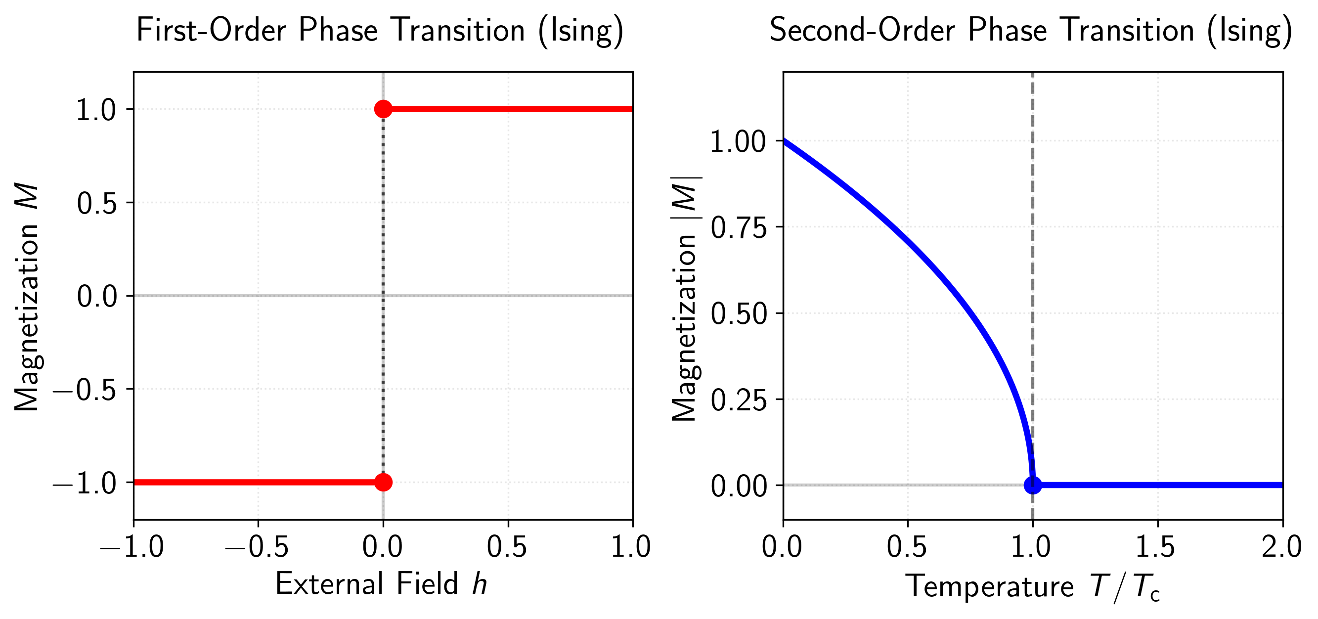
Figure 1: Comparison of first-order and second-order phase transitions in the Ising model. Left panel: First-order phase transition showing magnetization as a function of external field at . The magnetization exhibits a discontinuous jump from to at the critical point (dotted vertical line), demonstrating the discontinuity characteristic of first-order phase transitions. Right panel: Second-order phase transition depicting the absolute magnetization versus reduced temperature at zero external field. The magnetization follows the power law for and continuously approaches zero at (dashed vertical line), with critical exponent from the mean-field approximation.
Phase transitions occur at a critical point given by a co-existence curve (a sort of hyperplane) that separates two distinct phases of matter, such as water and ice. When crossing this boundary, the systems macroscopic properties change abruptly, whether through a first- or second-order phase transition. As the system size grows larger, approaching the thermodynamic limit, the properties on each side of this boundary become more sharply defined. This behavior is explained through renormalization group theory, which is a bit beyond the scope of this post, but I will refer to it once or twice more.
Throughout this post, we will use magnetism as the pedagogical example. At a microscopic level, magnetic materials derive their properties from the alignment of magnetic dipole moments. These moments arise primarily from the intrinsic spin of an electron, creating tiny magnetic fields that can interact with neighboring atoms. In ferromagnetic materials (such as iron), these dipole moments can align producing a permanent magnet. When a sufficient fraction of these magnetic moments align, they produce a net magnetic field. Here, we refer to magnetic materials as ferromagnet, and non-magnetic materials as paramagnets.
To give a concrete example of a phase transition that’s relevant within the context of this blog post, let’s consider the ferromagnet-paramagnet phase transition. The magnetization curve shown in Figure 2 illustrates the temperature dependence of the order parameter in a ferromagnetic system. For temperatures below the critical temperature (called the Curie temperature), the system exhibits spontaneous magnetization, represented by the two symmetric branches of the curve. These branches emerge from a bifurcation at and grow in magnitude as temperature decreases, following the power law , where is the critical exponent (which is something we will discuss later). The dashed line at for represents an unstable state, while the continuation above represents the paramagnetic phase where the thermal fluctuations overcome the ordering tendency of the magnetic interactions resulting in the loss of magnetization.
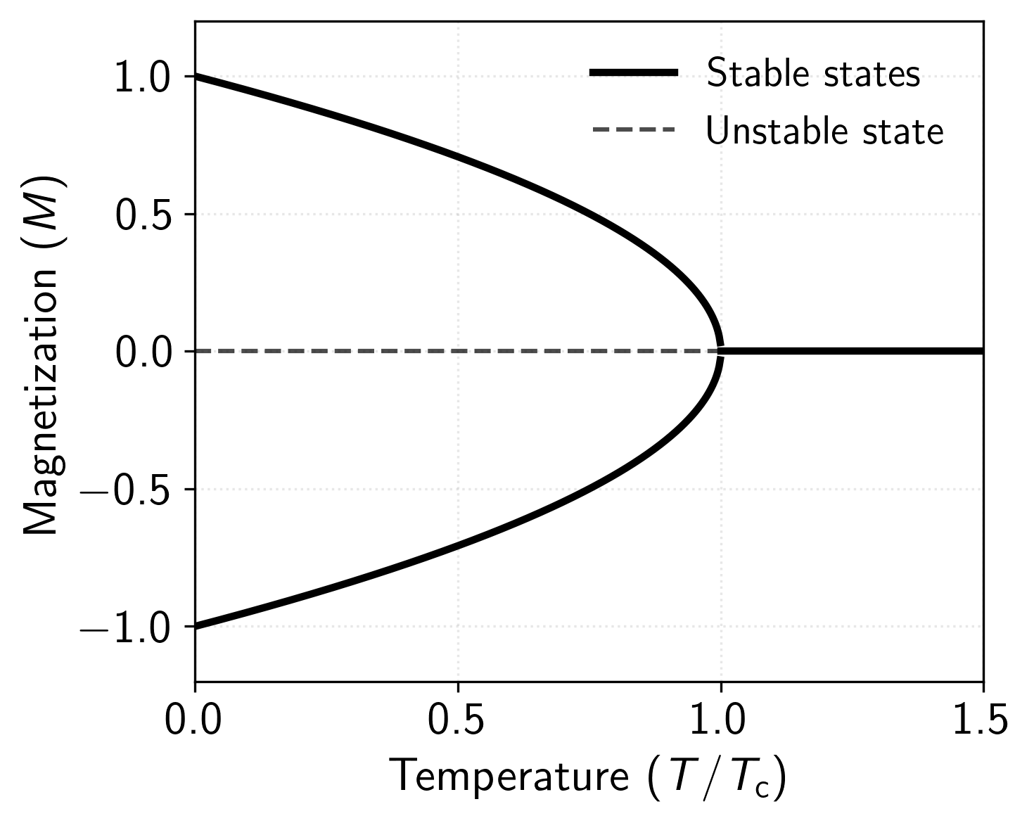
Figure 2: Phase diagram of the Ising model showing magnetization () as a function of reduced temperature ().
The first phase transition occurs as we vary the temperature with no external magnetic field present. Consider a permanent magnet at room temperature (such as iron) where the magnetic moments align themselves spontaneously in the same direction, creating a net magnetic field. As we heat this magnet above , it undergoes a dramatic change where the thermal energy becomes strong enough to overcome the alignment of these magnetic moments, and the material transitions into a paramagnetic phase where the magnetic moments point in random directions, resulting in no net magnetic field. This is a continuous or second-order phase transition where the magnetization gradually decreases to zero as we approach the critical temperature (Figure 1 above).
The second type of transition becomes apparent when we apply an external magnetic field at a fixed temperature below . Starting with a strong field in one direction, the magnetic moments align with this field. As we decrease the field strength to zero and then increase it in the opposite direction, the magnetization shows a sudden jump or discontinuity as it switches direction, characteristic of a first-order phase transition. Although, it is also worth noting that because all of the spins are aligned in one direction, there is a phenomenon called hysteresis, which is a sort of lag that occurs due to the spins not wanting to flip even if the external field flips. In this sense, the system’s response depends on its history, and hysteresis reflects the system’s preference to maintain alignment among its magnetic moments even as the external field reverses.
Critical Exponents and Universality
One interesting property of continuous phase transitions is that they exhibit a characteristic power-law behavior in various thermodynamic quantities as the system approaches some critical point. These power laws are characterized by critical exponents, which quantify how physical observables scale with the distance from the critical point. For a magnetic system at temperature near its critical temperature , we define the reduced temperature as a measure of this distance.
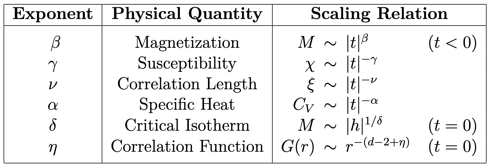
Table 1: Primary critical exponents and their associated scaling relations. Here, denotes the reduced temperature, the external field, and the spatial dimension.
This critical behavior is described by a set of critical exponents, each associated with a specific thermodynamic quantity. For example, the magnetization , below , scales as . Similarly, the magnetic susceptibility diverges as . These power laws characterize the singular behavior near the critical point, and can be observed across a wide range of (surprisingly different) physical systems. A larger set of the primary critical exponents and their scaling relations are presented in Table 1 above, and a more graphical plot can be seen in Figure 3 below.

Figure 3: Critical behavior of thermodynamic quantities in the 2D Ising model as functions of the reduced temperature . Left panel: The magnetization for with critical exponent (= 1/8), showing how the order parameter continuously approaches zero as the critical temperature is approached from below. Center panel: The correlation length with critical exponent , diverging at , which indicates the emergence of long-range correlations at the critical point. Right panel: The magnetic susceptibility with critical exponent (= 7/4), demonstrating the divergence of fluctuations near the critical point. These precise critical exponents are characteristic of the 2D Ising universality class and illustrate how different physical observables exhibit power-law behavior near the critical point, with exponents that are related through scaling relations.
The concept of universality as it relates to critical phenomena states that systems with distinct microscopic interactions, characterized by their (potentially very different) Hamiltonians, can exhibit identical critical exponents. This universal behavior can be understood through the role of fluctuations and the divergence of the correlation length near the critical point (more on correlation functions in the next section). When becomes much larger than any microscopic length scale, fluctuations on all length-scales become increasingly important, and the individual microscopic interactions becomes irrelevant to the critical behavior. These large fluctuations sort of wash out the microscopic details, leaving only the fundamental symmetries and dimensionality to determine the critical behavior. Systems that share these basic properties form a universality class, characterized by their identical critical exponents.
To give a concrete example, the liquid-gas critical point and the ferromagnetic phase transition in the three-dimensional Ising model have the same critical exponents, and are thus in the same universality class. This is despite the (large) differences in their microscopic physics, where one involves molecular interactions in a fluid and the other involves magnetic moments on a lattice.
Correlation Functions
To understand critical behavior, it’s going to be useful to have an idea for what form the spatial correlation function takes on. Consider a magnetic system where represents the local spin at position . The two-point correlation function is defined as
Where this function measures the degree to which fluctuations at different points in space are correlated, after subtracting out the effects of the average magnetization. For translationally invariant systems, this depends only on the relative displacement , allowing us to rewrite as . Away from criticality, this correlation function exhibits exponential decay
To understand why this is, consider a system with local interactions. The correlations between distant points must be built up through a chain of intermediate interactions. Each “step” in this chain introduces a multiplicative factor. The accumulated effect over a distance naturally leads to an exponential decay, with characterizing the typical distance over which correlations persist. However, what is very important to note is that at the critical point, the correlation function transitions to a power-law decay
where is the spatial dimension and is the anomalous dimension. Where the anomalous dimension is a sort of correction term that represents how the spatial correlations deviate from what would be expected in a simple non-interacting or mean field system, due to the critical fluctuations. This transition from exponential to power-law behavior reflects the emergence of scale invariance at criticality, as the divergence of eliminates the characteristic length scale that gave us the exponential decay.
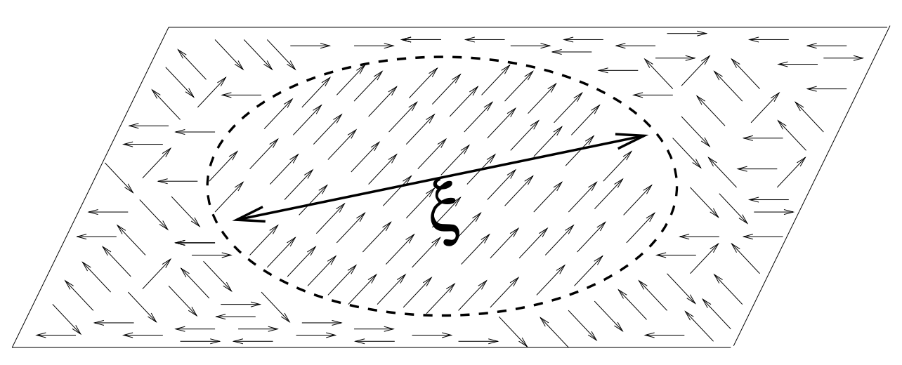
Figure 4: Visualization of the concept of correlation length. The figure depicts a 2D plane in 3D space with randomly oriented spins (represented by arrows) distributed throughout. Within a circular region of diameter , all spins are aligned in the same direction, while outside this region, spin orientations are random and uncorrelated. The correlation length defines the characteristic spatial scale over which the system maintains order. Spins separated by distances less than tend to be correlated, while those separated by distances greater than tend to behave independently. As the temperature approaches the critical point , this correlation length diverges according to , leading to long-range order and scale-invariant behavior characteristic of second-order phase transitions.
This is very interesting because it implies that systems that undergo a second-order phase transition have scale-free dynamics at the critical point. Within the context of a future post on the critical brain hypothesis, this is of interest because it explains why observing scale-free dynamics, in for example the size and lifetime distribution of neuronal avalanches, provide evidence for the brain operating near a second-order phase transition between ordered and disordered states. I’ll post more on this another time, but it also adds intuition for why the brain might want to self-organize or fine-tune near the critical point. That is, at the critical point there is a divergence in the correlation length allowing for optimal message passing between pairs of neurons.
The complete theoretical understanding of this power-law behavior emerges from the renormalization group analysis. Furthermore, the full derivation of the correlation function forms can be followed from the Ornstein-Zernike theory of correlation functions, which is slightly beyond the scope of this post. The Berlinsky [4] book has a good discussion of this in Chapter 13.
The Scaling Hypothesis
It turns out that the various critical exponents introduced in the previous section are not all independent. The scaling hypothesis, one of the fundamental principles in the theory of critical phenomena, asserts that only two of the critical exponents are independent, and that the remaining exponents can be determined through a set of scaling relations. The most fundamental of these relations are the Rushbrooke and Widom scaling laws
Further scaling relations can be derived by considering the role of the spatial dimension and the anomalous dimension . These relationships, known as the hyperscaling relations, and take the form
The existence of these scaling relations reveals a sort of simplicity underlying critical phenomena. Despite the complexity of microscopic interactions, systems near criticality can be characterized by just a few independent parameters. This reduction in complexity suggests that the behavior at critical points is not dependent on the specific details of the microscopic interactions, providing further support to the concept of universality discussed previously.
While I didn’t provide a full derivation of the scaling relationships, a thorough and pedagogical treatment can be found in Kopietz’s “Introduction to the Renormalization Group,” particularly in sections 1.2 and 1.3.
The Ising Model
The Ising model, often referred to as the Drosophila of statistical mechanics, is an abstraction of the microscopic properties of magnetism through discrete magnetic dipole moments (spins) that can either point up () or down (). More formally, the Ising model is defined on a -dimensional lattice where at each site there is a discretized abstraction of the spin . When the spins align we have a net magnetic field. When the spins do not align, they cancel each other out resulting in no net magnetization. Most important to our study of the Ising model in this post is the existence (or lack thereof depending on the dimensionality of the system) of first- and second-order phase transitions in the order parameter (magnetization) as we vary various control parameters (e.g., the strength of the external field or the temperature respectively).

Figure 5: Left: Random spin configuration in a 2D Ising model lattice at high temperature, exhibiting disorder with no clear pattern of aligned spins. Right: Low-temperature configuration showing two distinct magnetic domains separated by a well-defined domain wall. The left domain consists predominantly of -1 spins (light), while the right domain contains mostly +1 spins (dark), illustrating the spontaneous symmetry breaking and phase separation characteristic of the ferromagnetic phase below the critical temperature.
In the ferromagnetic phase below the critical temperature , the system spontaneously breaks symmetry as spins collectively align, forming clusters of uniform magnetization called magnetic domains. In real systems, these domains form due to competing interactions, boundary effects, and non-equilibrium dynamics. The boundaries between oppositely aligned domains are called domain walls (see Figure 5 above or the cover for this post), which have a characteristic width and energy cost (an interesting area of research). As temperature increases toward , thermal fluctuations cause these domain walls to become increasingly irregular and fluid. At the critical point, the correlation length diverges, meaning that fluctuations occur at all length scales, which dissolves the distinct domains as the system transitions to the paramagnetic phase.
Solving a Thermodynamic System
Before we go any further, it might be worth noting what the goals are, and what exactly it means to solve a system like the Ising model. First, we are interested in computing the mean magnetization of the spins , which is computed at the ensemble/thermodynamic mean of the individuals spins
Where are the possible micro-states of the system, and are the Boltzmann probabilities. These probabilities depend on the energy of each microstate, which is given by the Hamiltonian of the system. The Hamiltonian encodes all interactions and external influences in the system, and evaluating it for a particular microstate gives us the energy .
Following the principles of statistical mechanics, lower energy states are assigned higher probabilities than higher energy states according to the Boltzmann distribution
Where is the thermodynamic beta, is the Boltzmann constant, and is the Partition function (a normalization factor to ensure the probabilities sum to one). We are working in the canonical ensemble, which is a system at thermodynamic equilibrium with a reservoir heat bath, and so the canonical partition function is given by
The Helmholtz free energy of the system is related to the Partition function as
From the free energy, we can find most of what we are interested in. That is, the mean magnetization is related to the free energy as , and the magnetic susceptibility is , which refers how much the magnetization changes with the external field . And so in some sense, we are mainly interested in the free-energy of the system and it’s various derivatives, which we can get by computing the Partition function. Thus, to solve a thermodynamic system like this roughly boils down to computing the Partition function .
The Ising Hamiltonian
In true statistical mechanics fashion (I say this as someone who is not a Physicist), the first thing we will want to do is define the total energy of any state of the system, the Hamiltonian. To do so, notice that there are only two net forces on the system. Given any dipole moment , the forces acting on it are going to be the spins of it’s neighbors and that of any external magnetic field. First, we can model the neighboring interactions with the following term:
Where is the spin of the -th dipole, is the coupling strength between the -th and -th dipole, and the notation means to sum over all possible configurations of and . Notice that because of the symmetry with and in the notation, we also have a factor of one-half to account for the double adding of terms.
Next, we have the interaction of an external field on each dipole. This interaction can be written as
Where is the coupling of the external field on the -th dipole. Summing these two terms together gives us the Hamiltonian of the Ising model
Here, we will assume the traditional simplifications that and uniformly interact with all of the dipoles, and allow the one-half term to be absorbed by . This gives us the following simplified Hamiltonian which we will be working with for the rest of this blog post
Next, we will try and solve this system (compute the Partition function ) in a varying number of dimensions.
Exact Solution in Zero-Dimensions
In zero-dimensions, there is only a single spin and the interaction term in the Ising Hamiltonian vanishes, meaning that we are left with only the interactions between the spin and the external field . Therefore, in zero-dimensions our new Hamiltonian becomes
As previously mentioned, we must compute the partition function. Given there is only one spin with two possible states micro-states (), the Partition function can be trivially computed as
From this partition function, we can compute most of what we are interested in. First, the free energy is given by
The mean magnetization can be computed as the thermodynamic mean or expectation of the spin(s), which results in
Which is bounded strictly between and , dependent on the inverse temperature (assuming ) and the external field . Figure 6 below visualizes the mean magnetism (x-axis) at different temperatures. Given any non-zero external field, the average magnetism of the spin is always the sign of the external magnetic field. Right at zero external field, the mean magnetism is always zero (except for the divergence at absolute-zero, which we won’t worry about).
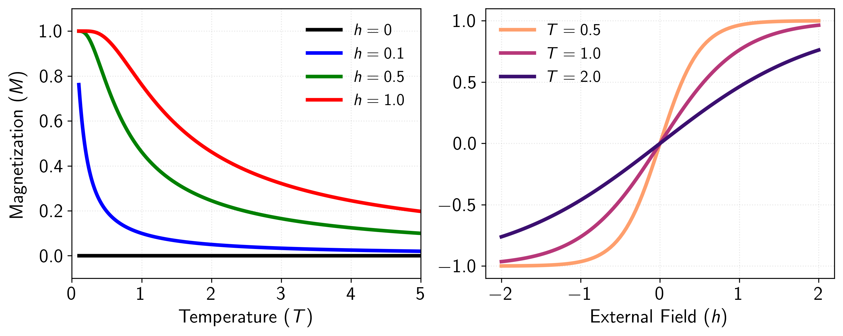
Figure 6: Zero-dimensional Ising model results showing the paramagnetic behavior of an isolated spin. Left panel: Magnetization as a function of temperature for various external field strengths. At zero field (), the magnetization is precisely zero at all temperatures due to the equal probability of spin up and down states. As external field strength increases (), the system exhibits induced magnetization that monotonically decreases with temperature. Right panel: Magnetization as a function of external field at different temperatures. The curves demonstrate the characteristic S-shaped response typical of paramagnetism, with steeper slopes at lower temperatures indicating higher magnetic susceptibility. As temperature increases, thermal fluctuations increasingly compete with the aligning effect of the external field, resulting in a more gradual approach to saturation.
The magnetic susceptibility , which measures the system’s response to small changes in the external field, can be derived from the average magnetization as
Meaning that while the zero-dimensional Ising model responds to external fields, it cannot exhibit a phase transition. The susceptibility remains analytical for all temperatures and fields, showing no divergence that would result in a phase transition.
Exact Solution in One-Dimension
In one dimension, the Ising Hamiltonian is given by
We define the periodic boundary condition converting this into a sort of circularly linked list. In the thermodynamic limit where , this shouldn’t matter too much, but it turns out that this assumptions affords us a couple of nice simplifications that makes the math easier later on.
Before computing the Partition function, let us first perform a change of variables
Where is the energy of the bonds between lattice sites and . Notice the factor of that snuck in due to the double counting of the external field energy.
Again, the partition function takes on the following form
Where are the possible states of the system. Notice that because we have interacting terms, this is already a lot harder of a partition function to solve than the zero-dimensional case. In my studies of this form, I came across two solutions: A combinatorial one, and one that involves a transfer matrix. I much prefer the latter, and so we will follow along with that solution. To do so, we will introduce a couple of notational tricks that allow us to rewrite the Partition function as a product of matrices (the transition matrix), which will result in a big simplification happening. First, let’s expand and simplify the Partition function a bit.
Where . Next, notice that can only take on four possible states: , , , and . Thus, we can represent the function with the following two-by-two (transfer) matrix
Where the value of is given by an element in , namely . Now, the key property that makes this technique so successful relies results from the following property
Which is just the definition of the matrix dot product. From this, we can simplify the partition function as
Because we are now only summing over , the only possible states left are and , which are the diagonal values of , or the trace.
The fact that we have a periodic boundary condition is really what enables the partition function to be written as the -th power of . This is a huge simplification, and has a closed form solution after eigenvalue analysis.
As a reminder, recall that the trace of a matrix is equal to the sum of its eigenvalues. Furthermore, because is symmetric and real, then is also, and that
Here, we define the eigenvalues as and , and assume that , then solve for them analytically. Also, note that because of the power of that we only care about the larger of the two eigenvalues since in the thermodynamic limit () we have
Setting up the characteristic equation and solving for and gives
Whose solutions (after setting to zero and solving for lambda) are
Now for the free energy, we want a system that is not proportional to N and so we instead define the free-energy per spin as . This gives us
Finally, taking the thermodynamic limit we get the final free-energy per spin as
Which evaluates to
After some tedious algebra, the magnetization per spin can be computed from the free energy as
At zero external field , analysis shows that for all . This absence of spontaneous magnetization indicates that the one-dimensional Ising model also cannot sustain long-range order at any non-zero temperature. The magnetic susceptibility can be computed by taking a second derivative
where is the effective field. This susceptibility remains finite for all non-zero temperatures, confirming the absence of a phase transition in the one-dimensional Ising model.
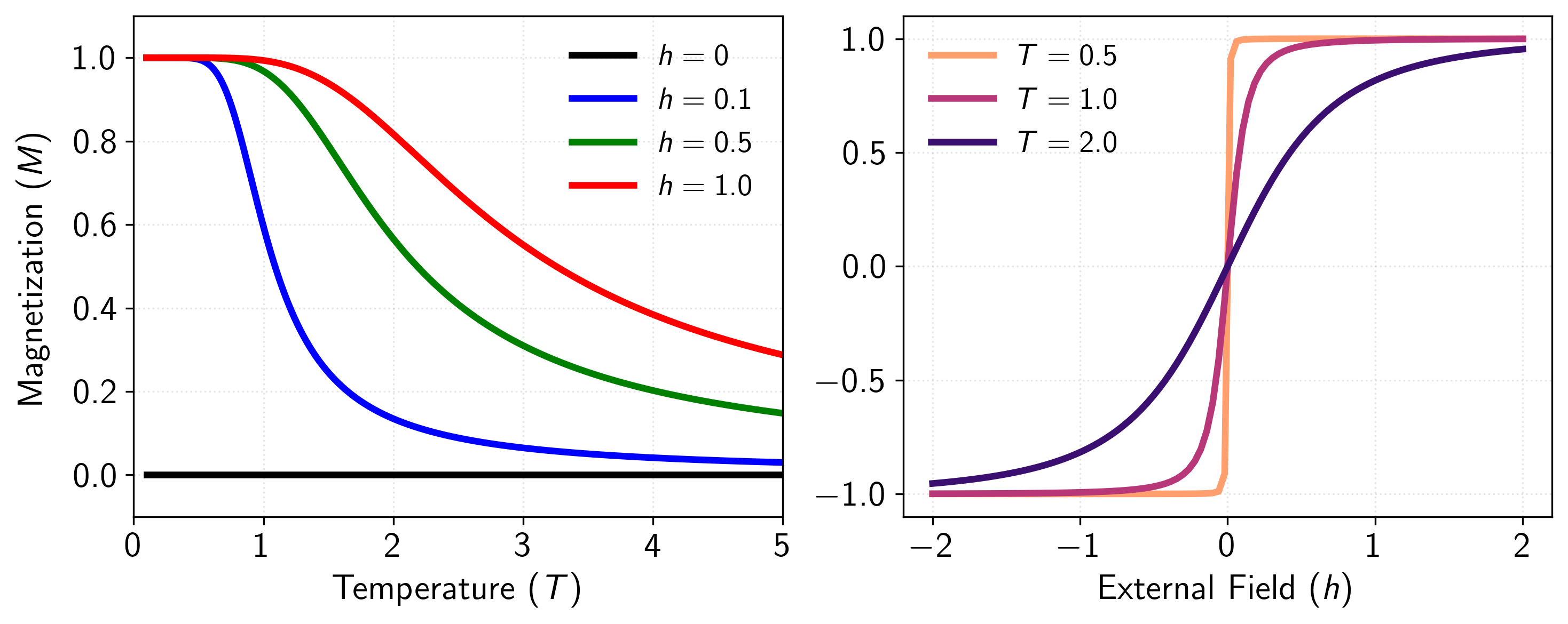
Figure 7: Magnetization behavior of the one-dimensional Ising model as a function of temperature for various external field strengths. At zero external field (), the magnetization remains exactly zero at all non-zero temperatures, demonstrating the absence of spontaneous magnetization in the 1D Ising model. This confirms the mathematical result that no phase transition occurs in the one-dimensional case, as the system cannot sustain long-range order at any finite temperature. As external fields of increasing strength () are applied, the system exhibits induced magnetization that asymptotically approaches zero at high temperatures as thermal fluctuations overcome the influence of both the external field and the nearest-neighbor interactions. The results are similar to the zero-dimensional case.
This lack of a phase transition in the one-dimensional Ising model is a result of the fact that the thermal fluctuations at any non-zero temperature are sufficient to destroy long-range order. That is, creating a domain wall in one dimension costs a finite amount of energy (), but the entropy gain from placing this domain wall anywhere along the chain grows logarithmically with system size. At any non-zero temperature, the entropic contribution to the free energy eventually dominates, favoring a disordered state. This competition between energy and entropy explains why higher dimensions are necessary for the existence of phase transitions at finite temperatures.
Mean Field Theory for -Dimensions
For the two-dimensional Ising model in the absence of an external field, there is a solution by Onsager [5], but it’s a bit too complicated to give the full derivation here. Instead, we will discuss an approximation of the Hamiltonian that will allow us to solve the Ising model in arbitrary dimensions, namely the mean field approximation. Unfortunately, this approximation leads to quite poor results for low dimensions, and actually breaks down right at the critical point which we’ll talk about later.
The goal of this approximation is to decouple interacting terms between neighboring spins by replacing them with a single interaction to the mean field. In doing so, we are able to convert the many-body problem (with many interacting spins) to a one-body problem where each spin only interacts with the mean field. But this often lends itself to a circular argument (called self-consistency) in which the dynamics of our new mean-field system rely on microscopic states, but the microscopic states rely now on the mean-field (rather than the individual terms). We will see this dependence appear later on.
Given the Hamiltonian of the Ising model in an arbitrary -Dimensions ()
and the magnetization of the system . We can then express the interacting spins as
In the mean field approximation, we neglect the correlation term because it represents fluctuations from the mean at different sites, which we assume to be uncorrelated and of higher order. This gives us the following new mean-field Hamiltonian
In dimensions, the number of neighbors each dipole on the lattice has is . Given this, the first term in the Hamiltonian becomes
And additionally, the second term becomes
Then, our mean-field Hamiltonian becomes
Where the effective field is the total magnetic field felt by the spins. In other words, we have essentially removed the pairwise spin-spin interactions, and replaced them with the effective field which consists of the external field and the mean field . Because all of the pairwise spins have been decoupled, the partition function becomes trivial to compute.
Notice that the swap of the product and sum above is possible because . Also note that the product came from the fact that , which is pretty trivial to see if you expand out the sum.
Then, the free energy per spin is
Remember that because we assume that , and thus the factors of cancel out in the left hand side of the free-energy. The behavior of the free energy for varying temperatures can be seen in Figure 8.
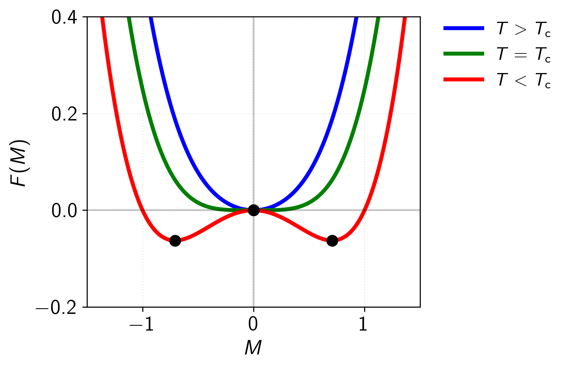
Figure 8: The characteristic shapes of the mean-field free energy at different temperatures. Above , the free energy has a single minimum at , reflecting the stability of the paramagnetic phase. At , this minimum becomes very flat, indicating the critical point where susceptibility diverges. Below , the free energy develops a characteristic double-well structure with minima at finite , corresponding to the two possible directions of spontaneous magnetization. The central maximum at represents the unstable state.
Now we can compute the magnetization as , which gives the self-consistency equation
To repeat what was said before, this is called the self-consistency equation because the mean-field relies on the microscopic states, but the microscopic states now also rely on the mean-field. That is, is a function of itself!
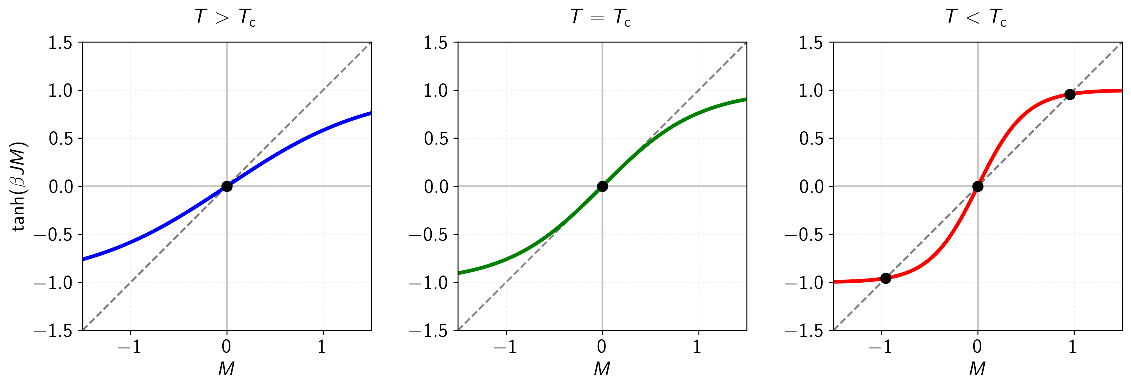
Figure 9: Graphical solutions to the self-consistency equation for the -dimensional Ising model in zero external field at different temperatures. The dashed line represents , while the colored curves show at three distinct temperatures relative to the critical temperature . Intersection points (black circles) indicate solutions to the self-consistency equation. Left panel (blue curve): For , only a single solution exists at , corresponding to the paramagnetic phase with no spontaneous magnetization. Middle panel (green curve): At , the slopes of the two curves match at , marking the critical point where the system transitions between ordered and disordered phases. Right panel (red curve): For , three solutions emerge: an unstable solution at and two stable solutions at , reflecting the ferromagnetic phase with spontaneous symmetry breaking. This graphical representation illustrates the emergence of non-zero spontaneous magnetization below as predicted by mean field theory.
To understand the phase transition in this mean field approximation, let us first determine the critical temperature by analyzing the self-consistency equation. At zero external field , we can examine when a non-zero magnetization first appears as we lower the temperature. For small , we can expand the hyperbolic tangent using its Taylor series
Truncating at the cubic term and substituting in gives
This equation has two types of solutions: (paramagnetic phase) and solutions where the term in square brackets vanishes (ferromagnetic phase). The critical temperature occurs when the coefficient of the linear term vanishes, and therefore
Above , only is stable. Below , non-zero solutions emerge, leading to the onset of spontaneous magnetization. More on the validity of these results in the next section.
Critical Exponents of the MFT Solution
Next, let’s derive some of the critical exponents to analyze how various quantities scale near . First, consider the magnetization below . As we did before, let’s define the reduced temperature , then notice that near we have
Substituting back into our expansion and rearranging gives
Which has a non-interesting solution at and another (more interesting) solution when the inner part is zero giving
Which for we have that or that with the critical exponent being . For the magnetic susceptibility, we can do something similar by differentiating the self-consistency equation with respect to resulting in
Given no external field and where we get roughly the following
This gives with . I skipped a couple of steps, but the whole derivation, and the derivation of some other critical exponents, can be found in Franz Utermohlen notes [6] on the topic, or either the Berlinsky [4] or Kopietz [7] books.
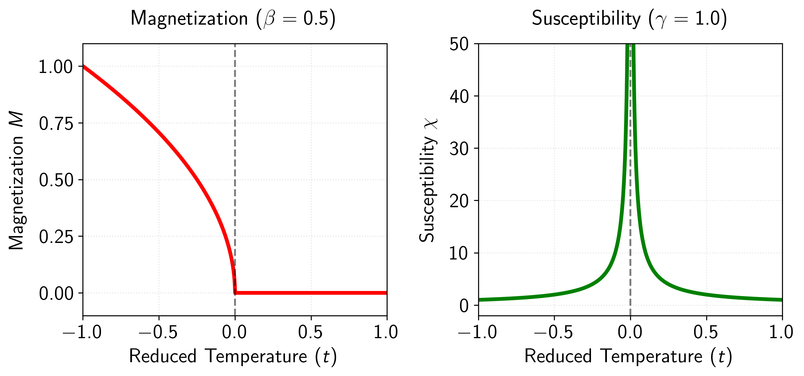
Figure 10: Critical behavior in mean-field theory (MFT) as a function of reduced temperature . Left panel: Magnetization with critical exponent . Right panel: Magnetic susceptibility exhibiting the power law divergence with critical exponent .
Remember that MFT gives us an approximate solution to the true Hamiltonian, so how good are these results? It turns out that in high dimensions, they are quite good (exact even), but fail in lower dimensions. Namely, above something called the upper critical dimension (where for the mean-field Ising model), fluctuations from the mean become irrelevant and these exponents are exact. Below , fluctuations modify the critical behavior in a way that mean field theory fails to capture.
For example, at zero external field (), this equation predicts a second-order phase transition at a critical temperature for all dimensions. The spontaneous magnetization below this temperature follows , with the critical exponent being independent of dimension. However, this contradicts our exact solutions for the 1D and 2D Ising model, where in one dimension, the transfer matrix method yields the exact partition function, showing that the free energy per site is analytic for all finite temperatures. The correlation length, given by , remains finite for all , demonstrating the absence of long-range order at any non-zero temperature.
Furthermore, in the two-dimensional case, Onsager’s exact solution shows that while a phase transition does exist, it differs significantly from the mean field prediction. The critical temperature in the exact solution () is lower than the mean field prediction of . More importantly, the magnetization near the critical point follows , with , rather than the mean field value of . We will talk further about these discrepancies in a couple of sections.
The Variational Principle
Next, I want to have a quick word about the theoretical basis for mean field theory, why it works, and present a quick relationship to variational inference. Recall that our goal from MFT is to simplify a many-body problem with interacting degrees of freedom into a more tractable one-body problem. In doing so, the (usually intractable) pairwise interactions are replaced by a single interaction between each degree of freedom and an effective “mean field.” In this sense, the first step in MFT involves replacing the original Hamiltonian , which encodes the full many-body interactions, with an approximate Hamiltonian. For consistency with standard nomenclature, we label this approximate form the trial Hamiltonian . Note that the trial Hamiltonian is just an approximation of the real Hamiltonian . Now, let be the partition function of in the canonical ensemble, and define the free energy to be the familiar
Which, for complicated with many interacting degrees of freedom, the problem of computing the partition function (), and thus the free energy (), is typically intractable. Here’s where the variational principle comes in. We introduce the trial Hamiltonian, , which ideally captures the essential features of while being much easier to handle. This trial Hamiltonian has its own partition function and free energy defined analogously. Then, the probability distribution associated with the trial Hamiltonian is
Now, we can derive the relationship between and as
This trial Hamiltonian allows us to rewrite the true free energy in a clever way by using this fact. Substituting back into the expression for , we find that
where is the expectation taken over the trial distribution . Simplifying this a bit further using Jensen’s inequality, which states that for a convex function like the logarithm, we get:
Where the right hand side of this inequality (called the Bogoliubov inequality) is called the variational free energy
This equation has a really nice interpretation. The first term, is the free energy of the trial Hamiltonian. The second term, , measures how much the trial Hamiltonian deviates from the true Hamiltonian , averaged over the trial distribution. Together they provide an upper bound on the true free energy . The optimal trial Hamiltonian is the one that minimizes this upper bound, bringing the approximation as close as possible to the true free energy.
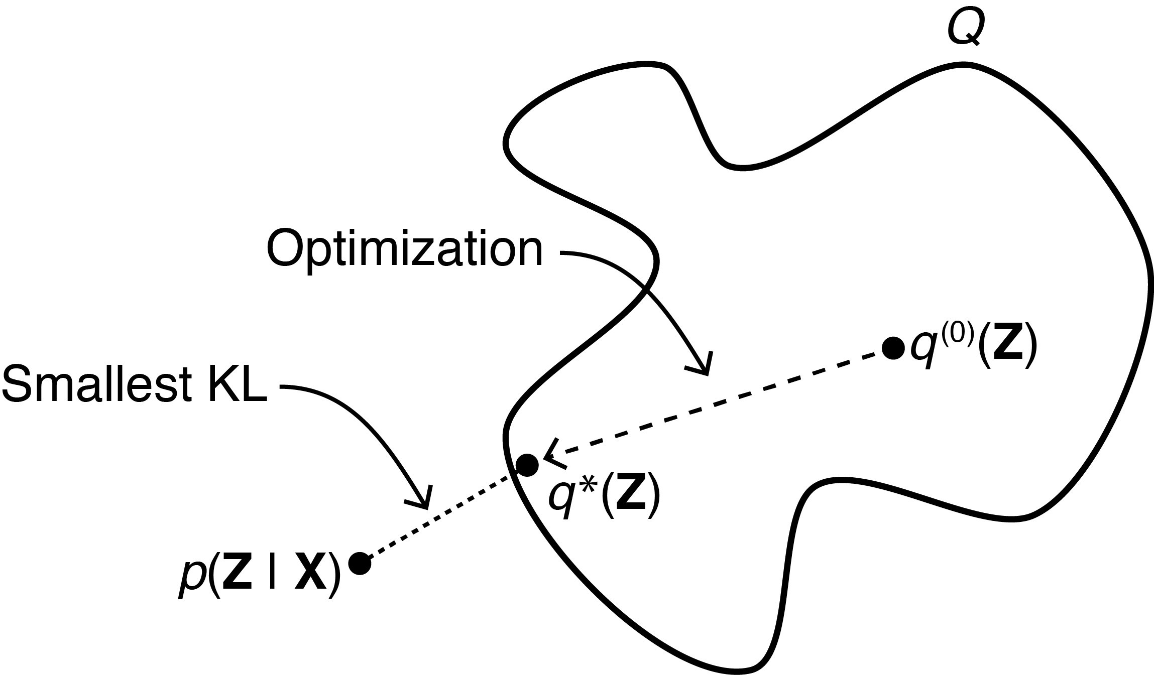
Figure 11: Image from Gregory Gundersen’s blog post on VI and the ELBO [8]. Schematic representation of the variational approach to mean field theory. The blob represents a family of trial distributions parameterized by the effective field. The optimization process starts with an initial trial distribution and iteratively minimizes the KL divergence between the current approximation and the true Boltzmann distribution . This process is equivalent to minimizing the variational free energy , which provides an upper bound to the true free energy according to the Bogoliubov inequality. The optimal distribution corresponds to the self-consistency equation in the Ising model, where the effective field parameter minimizes the difference between the trial Hamiltonian and the true many-body Hamiltonian .
The reason this is nice is because we essentially converted the mean-field problem into a variational inference one, where the closer is to , the closer the variational free energy becomes to the real free energy of the problem at hand. That is… if we parameterize with a set of weights, then optimizing over these weights is equivalent to making as small as possible… which causes to become a better approximation to … and thus approaches . And et voilà, it’s literally just variational inference. In fact, the Bogoliubov inequality is a sort of negative ELBO.
The see this briefly in play, let’s consider the generic Ising Hamiltonian again
Again, in the MFT approximation we want to remove the interacting terms and absorb them into an effective field, let’s now call .
Now, notice that is out parameter or weight we will optimize over. That is, we want to know the effective field that best approximates the true free energy given our MFT assumption. Plugging this into the variational free energy, computing the derivative, and optimizing for reveals
Which is just our self-consistency equation! Well, after substituting in the connection between the effective field and magnetism that is. Doing so gives
Super cool isn’t it! Now we have derived the self-consistency equation in two ways (albeit more in-depth in the former).
The Upper Critical Dimension
Recall that for MFT, we removed second order correlations between fluctuations, represented by terms of the form . While this approximation captures qualitative features of phase transitions, it fails to accurately predict critical exponents below a certain spatial dimension, known as the upper critical dimension . To determine , we can check the validity of MFT by examining the ratio of fluctuations to the square of the order parameter
This inequality must hold for the mean field approximation to be a good approximation. Near the critical point, we can express this ratio in terms of known quantities. The numerator, representing fluctuations about the mean, is related to the magnetic susceptibility , while the denominator scales as the square of the magnetization. Using our mean field results
Here, is the reduced temperature, and and are the mean field critical exponents.
These mean field exponents are modified by fluctuations. In general, fluctuations are controlled by the correlation length , which determines the size of correlated regions. The Ginzburg criterion states that mean field theory breaks down when fluctuations within a correlated volume become comparable to the square of the order parameter.
The correlation volume scales as , where is the spatial dimension. The magnitude of fluctuations within this volume can be derived from the two-point correlation function , which scales as at the critical point. Integrating over the correlation volume gives a typical fluctuation size of . Therefore
Using the mean field scaling relation , we obtain that
For mean field theory to become exact as (approaching the critical point), this ratio must vanish, requiring
This yields as the upper critical dimension for the Ising model with short-range interactions. For , fluctuations become irrelevant near the critical point, and mean field theory provides exact critical exponents. At , we find logarithmic corrections to mean field behavior where
For , the mean field description breaks down near the critical point, and we must use more sophisticated methods like the renormalization group to obtain correct critical exponents.
The physical intuition behind this dimensional dependence is that in higher dimensions, each spin has more neighbors (), making the mean field approximation more accurate as dimensionality increases. When , this effect is strong enough to suppress critical fluctuations entirely.
Specifically, MFT fails at the critical point because of the growing magnitude of fluctuations. As we approach , the correlation length diverges, meaning that spins become increasingly correlated over large distances. Mean field theory assumes that each spin feels only the average effect of its neighbors, effectively treating fluctuations as small and uncorrelated. However, near , fluctuations occur on all length scales up to , and these fluctuations are highly correlated.
In lower dimensions (), these correlated fluctuations become particularly important as the collective behavior of many spins moving together can no longer be approximated by independent spins responding to an average field. This collective behavior leads to different critical exponents than those predicted by mean field theory, requiring more sophisticated theoretical approaches.
Final Words
A bit of a longer post I guess, but I found this topic really interesting, and it’s been pretty widely studied so there is a lot of depth that can be explored. This post is basically just a dump of everything that I have been studying along this axis for the past couple of months. In fact, I could probably write another 20 pages on renormalization group methods, and it’s super interesting relationships to deep learning [9] [10] [11]. There have even been some people who have tried to take similar approaches to studying criticality [12], which I think is an interesting research direction. But, I will leave this for another time. There is just too much to write about, and to many things that I want to look into. Most likely the next post up will be on mechanistic interpretability, but we’ll see.
References
- Beggs, J. M. (2022). The Cortex and the Critical Point: Understanding the Power of Emergence.
- Beggs, J. M. (2022). Addressing skepticism of the critical brain hypothesis. Link
- Tian, Y., Tan, Z., Hou, H., Li, G., Cheng, A., Qiu, Y., Weng, K., Chen, C., Sun, P. (2022). Theoretical foundations of studying criticality in the brain. Link
- Berlinsky, A. J., Harris, A. B. (2019). Statistical Mechanics: An Introductory Graduate Course.
- Onsager, L. (1944). Crystal Statistics. I. A Two-Dimensional Model with an Order-Disorder Transition. Link
- Utermohlen, F. (2018). Mean Field Theory Solution of the Ising Model. Link
- Kopietz, P., Bartosch, L., Schütz, F. (2010). Introduction to the Functional Renormalization Group.
- Gundersen, G. (2021). The ELBO in Variational Inference. Link
- Mehta, P., Schwab, D. J. (2014). An exact mapping between the Variational Renormalization Group and Deep Learning. Link
- Bény, C. (2013). Deep learning and the renormalization group. Link
- Rojefferson (2019). Deep Learning and the Renormalization Group. Link
- Meshulam, L., Bialek, W. (2024). Statistical mechanics for networks of real neurons. Link
- Ising, E. (1925). Beitrag zur Theorie des Ferromagnetismus. Link
- Baxter, R. J. (2016). Exactly solved models in statistical mechanics.
- Sakthivadivel, D. A. R. (2022). Magnetisation and Mean Field Theory in the Ising Model. Link
Figures
- Custom. First- versus second-order phase transitions. Link.
- Custom. Magnetism phase diagram. Link.
- Custom. Critical exponents for magnetism, correlation length, and susceptibility. Link.
- From the Physics Stack Exchange. Illustration of the correlation length. Link.
- Custom. Illustration of the 2D Ising model on a lattice. Link.
- Custom. Zero-dimensional Ising solution. Link.
- Custom. One-dimensional Ising solution. Link.
- Custom. Free energy for the mean-field Ising model at various temperatures. Link.
- Custom. Visualization of the self-consistency equation at various temperatures. Link.
- Custom. Critical exponents for the mean-field Ising. Link.
- From Gregory Gundersen’s blog post on variational inference. Link.
Tables
- Custom. Various critical exponents.